| [PDF] |
|
| [PDF] |
|
For the purposes of the ILUTE land use/transportation model, most of the improvements described in Chapter 4 seemed promising for the synthesis of a population of persons, families, households and dwelling units. A sparse data structure was used, a hierarchy of margins were used to help with random rounding, and conditional synthesis was used to link the different types of agents. The PUMS simplification procedure would increase the memory requirements of the sparse data structure, and was not employed. The projection method for dealing with random rounding was not deemed a significant improvement over the conventional IPF procedure, and was also not used.
|
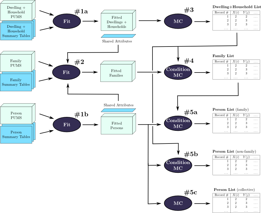
A complete overview of the population synthesis procedure is shown in Figure 5.1. The numbered steps shown in the figure are:
The method was implemented using special-purpose software written for the R/S+ statistical computing platform [29] with a few routines in C for additional speed. The following sections discuss the population universe, relationship model, population attributes, selection of shared attributes and software implementation.
The person, family and household universes are slightly reduced to match available data. No data is available on unoccupied dwellings, so only occupied dwellings are synthesized. This simplifies the dwelling/household relationship to a one-to-one mapping, allowing dwellings and households to be synthesized simultaneously. Almost no data is available on persons in institutions, so they are excluded from synthesis. Temporary, foreign and collective residents are included in most tables and are included in the synthesis for the purposes of accounting, but are not associated with any household, family or dwelling. For the fitting procedure, only persons 15 years of age and older are included, since most tables exclude younger persons. The conditional synthesis procedure does create persons under 15 years of age, but their only attributes are age and sex, since nothing further is available.
Finally, it is difficult to combine data from the 20% and 100% samples of
the person universe. Most tables are on the 20% sample and exclude
institutional residents, but the few that are defined on the 100% sample
include the institutional residents. There is very little data on the
institutional population, and they cannot always be removed from the 100%
sample to match the 20% universe. Since more data is available on the 20%
sample, it was used for synthesis, and the only 100% table used was
CF86A04 (
![]() );
DM86A01 was not used. The CF86A04 table was fitted to the 20% totals
for
);
DM86A01 was not used. The CF86A04 table was fitted to the 20% totals
for
![]()
For the family and household/dwelling synthesis, the 20% and 100% samples are defined on the same universe and are easier to combine. The 100% samples were used for both of these universes, which required a few 20% household table to be fitted to the 100% universe.
|
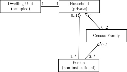
The relationships synthesized between the different agents/objects are shown in Figure 5.2. Each household consists of zero or more census families, and zero or more non-family persons. There are approximately 28,000 multifamily households in the Toronto CMA, accounting for 2.3% of all households and 4.7% of the population. Multifamily households are not particularly desirable from a modelling standpoint; they were not contemplated as part of the original ILUTE prototype, and their behaviour would be challenging to model. Nevertheless, to properly account for persons and families during the synthesis of the dwellings, families and persons, multifamily households must be included. There is no data on exactly how many households contain more than two families, but it can be estimated as approximately 1,000 of the 28,000 multifamily households5. For the purposes of synthesis, these are treated as two-family households.
Some of the non-family persons in a household may still form an economic family, and be related to other household members; as described in Chapter 3, 3.9% of the Toronto CMA population are non-family persons living with relatives. However, there is very little data on these persons and on economic families in general, although a patchwork of information can be gleaned from the Person PUMS and the Household PUMS. Furthermore, the economic family is not a particularly useful unit to synthesize from a behavioural perspective. While census families make many decisions as a unit (e.g., moving home or buying/selling vehicles), economic families are less unified in their behaviour. Elderly parents or married children living with relatives may choose to change homes or vehicle ownership independent of the other members of their economic family. In light of its limited usefulness and importance for the rest of synthesis, economic families were excluded from synthesis. Persons living with relatives are treated the same as other non-family persons.
Finally, each census family contains two or more persons (at a minimum, either a husband and wife or a lone parent and child). These relationships between agents can also be examined in the reverse direction. Each person is a member of zero or one census family, and is a member of zero or one household; each family belongs to a single household. (Persons in collective dwellings and institutions are the only persons who do not belong to a household.) Each household occupies a single dwelling unit.
The relationships (and universes) used for synthesis may not be ideal for the actual microsimulation model. The existing ILUTE and TASHA models do not define families as an explicit agent, but instead include family relationships as part of the household agent; they also did not allow for multifamily households. It is admittedly difficult to build behavioural models at the family level; the definitions of family relationships are sufficiently complex that few data sources are collected on the family universe. Even if more data was available, it is unlikely that the family definitions would be sufficiently consistent to be useful. Similarly, multifamily households are rare enough (and complex enough) that activity diary data is not always adequate to model their behaviour.
The synthesis here only accounts for some of the agents needed for the ILUTE microsimulation. Some of the other agents, objects and relationships can easily leverage this initial synthesis: household-level vehicle ownership, for example, can be readily modelled once the household composition is known. The combined synthesis of household vehicle ownership and location of work for multiple-worker households remains an important challenge, however, given the limitations of available data.
|
The categorization schemes in these data sources are often different, and some effort must be taken to establish suitable categorizations. A relatively fine categorization scheme was chosen for the source table during the IPF procedure, although not quite as fine as the PUMS categorization. The marginal tables generally had a coarser categorization for their attributes. To connect the two, mappings were constructed defining how the fine categories in the high-dimensional table could be collapsed to produce the coarser categorization in the marginal tables.
The final set of attributes synthesized during the IPF stage are shown in Table 5.1, along with the number of categories used in synthesis. Further details are shown in Appendix A.
For any group of agents linked through a relationship, the agents' attributes need to satisfy certain constraints, precluding impossible agent relationships such as a mother who is younger than her child. The method described in Chapter 4 was used to ensure that a selected set of agent attributes are consistent and follow an observed probability distribution. In brief, the stages of the method are:
This section focuses on the first step; the last two steps are described in detail in Chapter 4. The full set of shared attributes are shown in Table 5.2, and explained in the remainder of this section.
The household/dwelling linkage was easy and automatic, thanks to the one-to-one relationship between occupied dwellings and households and the existence of a single PUMS combining both sets of attributes. Consistency between related household attributes (e.g., HHSIZE), dwelling attributes (ROOM) and combined attributes (PPERROOM) was automatic, since all data in the Household PUMS is consistent.
The family/person linkage was fairly straightforward to select and construct. There are clear constraints between the family members that need to be preserved: for example, the age of the parents relative to the children and similarity in the parents' ages. To enforce such an age constraint, an age attribute must be present on both family and person agents, and the agents must agree on the distribution of ages. On the family agent, the attribute can be explicit like AGEF and AGEM (the husband/wife ages) or implicit like CHILDA (the number of children in the family of age 0-5).
The second obvious candidate for a constraint within the family is the labour force activity attribute. The presence of young children has a strong effect on the parents' labour force activity, and the two parents' activity is correlated. As a result, AGEP, LFACT, SEXP and CFSTAT are the obvious candidates for linkage attributes, and are included (directly or indirectly) on both the family and person agents. This matches the set of constraints applied by Arentze & Timmermans [2] in their synthesis of households.
Other person attributes such as highest level of schooling (HLOSP) or occupation (OCC81P) are also likely to exhibit correlation between husband and wife, but are not deemed critical for the ILUTE model. For a transportation model, the travel to work associated with labour force activity is more critical. Because HLOSP and OCC81P are not treated as shared attributes, the association pattern between the husband and wife may not be accurate for these attributes.
The household/family linkage was the most challenging in this dataset. There were three primary options for performing the linkage, which could be used independently or combined:
Initially, the household maintainer looked like an appealing link, since it would allow a single set of attributes to be shared between the three types of agents; perhaps the maintainer's age and labour force activity could be carried throughout. However, the definition of the maintainer is too open-ended to be consistently useful. In 4.9% of households including census families, a child or non-family person is the maintainer; little or no demographic information about these persons is present in the Family PUMS, making linkage difficult. Additionally, in multifamily households the maintainer demographics only give information about one of the families.
Dwelling/household characteristics are more usable for linkage. Given the importance of the housing market to the ILUTE model, it is vital
to ensure that families occupy legitimate dwellings, particularly homes
that are large enough. The HHSIZE attribute combined with the
ROOM attribute in the Household PUMS can ensure that the dwelling
has enough rooms to accommodate the persons in the household. The Family
PUMS includes a CFSIZE attribute; if it can be guaranteed that
![]() , then the family can fit in the dwelling.
However, families can share rooms in a dwelling in a different manner from
unrelated persons. The ROOM attribute is one of the few household/dwelling
attributes present in the Family PUMS, and is the only data available
showing how families use dwelling space differently from non-family
households. Finally, the tenure TENURH also provides an important
link with parents' ages. These two attributes were ultimately
chosen to define the dwelling/family link, with an additional special
constraint between ROOM, family size CFSIZE, HHSIZE and
the number of families
HHNUMCF.6
, then the family can fit in the dwelling.
However, families can share rooms in a dwelling in a different manner from
unrelated persons. The ROOM attribute is one of the few household/dwelling
attributes present in the Family PUMS, and is the only data available
showing how families use dwelling space differently from non-family
households. Finally, the tenure TENURH also provides an important
link with parents' ages. These two attributes were ultimately
chosen to define the dwelling/family link, with an additional special
constraint between ROOM, family size CFSIZE, HHSIZE and
the number of families
HHNUMCF.6
Financial attributes are also a possible link and a useful constraint, but were not pursued in this work. From a modelling standpoint, it would be valuable to be able to ensure that the members of a household have an income sufficient to pay the rent/mortgage for the dwelling they occupy. However, due to the large number of persons (both family and non-family) potentially involved in this relationship, it would likely be tricky to implement.
The final linkage is between household and non-family persons, and it is trivial: only the family status attribute on the person is used to link these two levels. Non-family persons are assumed to be independent of each other, and are hence synthesized independently and attached to the household.
There are a few constraints that would be useful to apply to non-family persons. Non-family persons under 15 years of age are more likely to live in a household that has at least one family, rather than living in a household of unrelated adults. Additionally, as discussed in Chapter 3, the census codes many same-sex couples as cohabiting non-family persons. The underlying data does not provide any information about the distribution of genders and ages of non-family persons sharing a dwelling, however, so no constraints can be applied.
The population synthesis procedure was implemented in the R language [29]. R is a statistical computing platform whose syntax closely resembles S [3], but with an underlying implementation borrowed from the Scheme and Lisp languages. It was selected largely because of good performance, concise syntax, a good set of built-in routines for analyzing and visualizing categorical data and multiway contingency tables, and built-in log-linear and generalized linear models. While it was suitable for prototyping and experimenting with new methods, its data storage is not efficient for large amounts of data, and its performance is poorer than low-level languages like C.
The central components of the software are a sparse list-based implementation of the Iterative Proportional Fitting algorithm, and a sparse list-based conditional Monte Carlo procedure.
The implementation of the Iterative Proportional Fitting procedure largely
followed the description in Chapter 4. Its inputs include a
list-based representation of a PUMS (in the R environment, this is called a
data frame), a list of marginal constraints, a termination tolerance
![]() and an iteration limit. The marginal constraints are complete
multiway contingency tables, which are associated with columns in the PUMS
through the use of standardized variable names. Each constraint can also
include a category mapping scheme, defining how the PUMS categories need
to be collapsed in order to match the category system used by the margin.
and an iteration limit. The marginal constraints are complete
multiway contingency tables, which are associated with columns in the PUMS
through the use of standardized variable names. Each constraint can also
include a category mapping scheme, defining how the PUMS categories need
to be collapsed in order to match the category system used by the margin.
Marginal constraints are applied in series, in the conventional manner for IPF. This does mean that the result is slightly dependent on the order that the constraints are applied; typically, the final constraint achieves perfect fit while earlier constraints do less well. Dykstra's suggestion of a parallel update procedure [17] is worth considering as an alternative.
A small part of the IPF procedure was implemented in C for performance reasons: collapsing the sparse list down to the marginal dimensions, and applying the marginal update back to the weights in the sparse list. The R language provided adequate performance for the other parts of the procedure.
To deal with random rounding, the modified IPF termination criterion described in Chapter 4 was employed. Additionally, the full hierarchy of margins was used to reduce rounding error in aggregate tables.
The data did include some area suppression, but a small amount of data was available to estimate the bare minimum information for these zones: the total population. The suppressed areas were assumed to follow the PUMA average distribution for each margin, scaled to the appropriate total population.
As discussed in Chapter 4, ordinary Monte Carlo
synthesis can easily be implemented using a sparse data structure, and
conditional synthesis is only slightly more complicated. Suppose attributes
![]() and
and ![]() are given, and attribute
are given, and attribute ![]() needs to be synthesized using a
joint probability distribution
needs to be synthesized using a
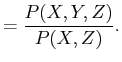
joint probability distribution ![]() . Then, the formula for
conditional probability is
. Then, the formula for
conditional probability is
 |
(27) |
The rest of the algorithm was simple to implement, and the complete details
are shown as pseudocode in Figure 5.3. The overall performance
is
![]() , and the operation was also implemented in C to
improve performance.
, and the operation was also implemented in C to
improve performance.
Some authors have used other versions of Monte Carlo, such as drawing without replacement [26,28]. In such approaches, after making draw a particular agent from a table of counts, the corresponding cell is decremented by 1 to prevent synthesis of too large a number of persons of any particular type.
These techniques have little or no value for this dataset, because the number of cells with counts greater than or equal to 1.0 is very small; almost all cells have fractional counts less than 1. For example, in the population of 2.7 million persons, only 20,090 persons are synthesized from cells with counts greater than or equal to 1.0.
| ||||||||||||||||||||||||||||||||||||||||||||||||||||||||||||
The final population was synthesized for the Toronto Census Metropolitan Area using the associated PUMS datasets. The compute times for population synthesis are substantial, but not extravagant. As shown in Figure 5.3, the synthesis required two hours and seven minutes to complete on an older 1.5 GHz computer with 2GB of memory. Synthesis of this duration is not a major issue since it can be performed once before a set of ILUTE model runs (or once per run, if different populations are desired), and the ILUTE model itself is considerably more compute-intensive.
Finally, the process was repeated for other CMAs using their own PUMS data: the Hamilton CMA was synthesized together with the Kitchener and Niagara-St. Catharines CMAs (since these three CMAs had a single shared PUMS in 1986), and the Oshawa CMA was also synthesized. Oshawa did not have its own PUMS in 1986, so the Toronto PUMS was used instead. Together, these three CMAs form the Greater Toronto/Hamilton Area, the urban region that the ILUTE project aims to study.
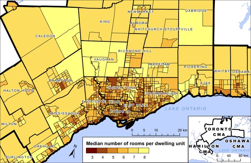
Using this population, any number of cross-tabulations and maps can be produced. To give a sense of the geography, Figure 5.4 shows a map of the median number of rooms in the dwelling units in each census tract in the Toronto CMA. This data is not available in any existing summary tables, although one table shows household size by zone and another shows persons-per-room by zone. Without any ground truth, the result cannot be verified, but it does match local general knowledge of dense and/or high-rise neighbourhoods. In particular, the zones with the lowest median number of rooms (smallest dwellings) are known to contain a large number of tall apartment buildings (often social housing) or student residences. One surprising zone with a median of 3 rooms per dwelling occurred in rural Niagara, but proved to contain largely “movable dwellings,” which are otherwise rare in the Toronto area.
![\begin{algorithm}
% latex2html id marker 4218
[tb]\KwIn{List $\mathbf{W}$\ con...
...thod can be easily generalized to a large number of attributes.}
\end{algorithm}](img308.png)