| [PDF] |
|
| [PDF] |
|
The existing population synthesis procedures have many limitations. In this chapter, the following concerns are discussed:
The chapter is structured largely as a discussion of these issues, together with an attempt to brainstorm solutions to these limitations, focusing particularly on the IPF-based methods; not all ideas are entirely successful. The new methods are intended to be largely independent, but most can be combined if desired. In the following chapters, several of these new methods are implemented and evaluated.
The IPF method has been applied to tables with a large number of
dimensions, as many as eight. Such high dimensional tables are almost always sparse, with the vast
majority of the cells in the table containing zeros. (High dimensional
tables are generally notorious for their difficulties and differences from
two-dimensional tables; see [12] for “ubiquitous”
ill-behaved examples.) In these sparse tables,
a large fraction of the non-empty cells contain only one observation, and
the number of cells is often much larger than the number of observations. In
other words, the sample does not provide a statistically meaningful
estimate of the probability distribution for such a high dimensional table.
However, the high-dimensional table can be collapsed to produce 2D or 3D
tables, each of which is adequately sampled and gives a statistically valid
distribution of counts. This is illustrated in Table 4.1,
where 99.7% of the cells are zero in the 8-way table. The two-way and
three-way margins of the table shown (
![]() and
and
![]() ) have 0% and 5.6% zeros, and
median cell counts of 90 and 30 respectively. Of course, an 8-way table has
many other lower-dimensional margins, and only one such choice is
illustrated in Table 4.1. (When collapsing a
) have 0% and 5.6% zeros, and
median cell counts of 90 and 30 respectively. Of course, an 8-way table has
many other lower-dimensional margins, and only one such choice is
illustrated in Table 4.1. (When collapsing a ![]() -way table to
-way table to
![]() dimensions, there are
dimensions, there are
![]() possible choices of variables to
keep in the low dimensional table.)
Consequently, while a sparse 8-way table does not provide statistically
testable 8-variable interaction, it could be viewed as a means of linking
the many 2- or 3-way tables formed by its margins.
possible choices of variables to
keep in the low dimensional table.)
Consequently, while a sparse 8-way table does not provide statistically
testable 8-variable interaction, it could be viewed as a means of linking
the many 2- or 3-way tables formed by its margins.
The cell counts in the high dimensional table say very little statistically; in fact, half of the non-zero cells contain just one observation. The most important information in an 8-way table is not necessarily the counts in the cells, but rather the co-ordinates of the non-zero cells, which determine how each cell influences the various low-dimensional margins. In this manner, the importance of the high-dimensional table is in many ways its sparsity pattern, which provides the link between the many 2- and 3-way tables. However, the sparsity pattern in the high dimensional table is in some ways an artefact of sampling. Some of the zeros in the table represent structural zeros: for example, it is essentially impossible for a family to exist where the wife's age is 15, her education is university-level and the family has eight children. Other zeros may be sampling zeros where the sample did not observe a particular combination of variables, but it does exist in the population.
All of the population synthesis strategies reviewed in Chapter 2 preserved the sparsity pattern of the high-dimensional PUMS. It would be useful if the synthesis procedure could account for the uncertainty surrounding the sparsity pattern. One strategy for resolving this would be to simplify the PUMS, building a variant that fits the low-dimensional margins but makes no assumptions about the associations or sparsity pattern in high dimensions where sampling is inadequate. The primary goal would be to correct sampling zeros in the high-dimensional PUMS, replacing them with small positive counts.
|
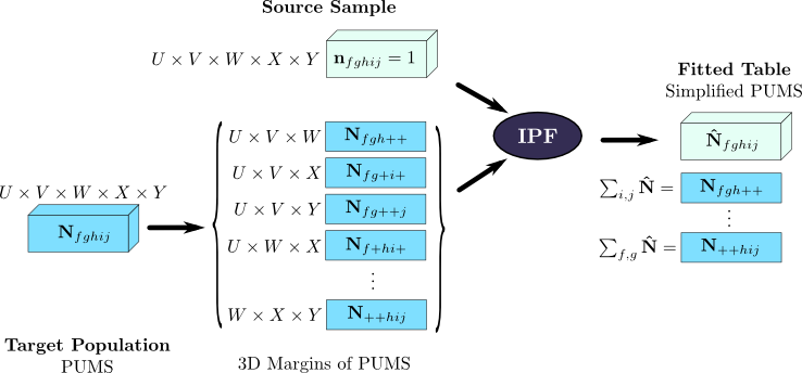
This strategy is illustrated in Figure 4.1. IPF is
applied on a high-dimensional table, with the source sample set to a
uniform distribution. The constraints applied to IPF are the full set of
(say) 3-way cross-tabulations of the PUMS. For a 5-dimensional problem,
this is equal to
![]() separate constraints. After IPF, the
simplified PUMS matches all of the 3-way margins from the PUMS, but
includes no 4-way or 5-way interaction between variables. In this example,
a 5-way table is shown for illustration, but the intention is for
higher-dimensional tables to be simplified. Also, 3-way margins of the PUMS
are used as constraints for illustrative purposes, but the actual margins
chosen could be selected using tests of statistically significant
interaction; If a log-linear model shows some significant 4-way interactions
in the PUMS, then these could be included as margins.
separate constraints. After IPF, the
simplified PUMS matches all of the 3-way margins from the PUMS, but
includes no 4-way or 5-way interaction between variables. In this example,
a 5-way table is shown for illustration, but the intention is for
higher-dimensional tables to be simplified. Also, 3-way margins of the PUMS
are used as constraints for illustrative purposes, but the actual margins
chosen could be selected using tests of statistically significant
interaction; If a log-linear model shows some significant 4-way interactions
in the PUMS, then these could be included as margins.
This method does indeed reduce the number of zeros in the high-dimensional table, correcting for sampling zeros and capturing some unusual individuals that were not included in the original PUMS. However, this strategy has significant downsides. In particular, it makes no distinction between structural and sampling zeros at high dimensions: there may be structural zeros involving four or more variables that do not appear in 3-way tables, but they will be treated the same as sampling zeros and be filled in with small positive counts.
Furthermore, it makes the entire population synthesis procedure more difficult, since agents can be synthesized who did not exist in the original PUMS. This makes the technique difficult to combine with some of the other methodological improvements discussed here.
For a microsimulation model spanning many aspects of society and the economy it is useful to be able to associate a range of attributes with each agent. Different attributes are useful for different aspects of the agent's behaviour. For a person agent, labour force activity, occupation, industry and income attributes are useful for understanding his/her participation in the labour force. Meanwhile, age, marital status, gender and education attributes might be useful for predicting demographic behaviour.
However, as more attributes are associated with an agent, the number of
cells in the corresponding multiway contingency table grows exponentially.
A multiway contingency
table representing the association pattern between attributes has
![]() cells. If a new attribute with
cells. If a new attribute with ![]() categories is added, then
categories is added, then ![]() times more cells are needed. Asymptotically,
the storage space is exponential in the number of attributes. As a result,
fitting more than eight attributes with a multizone IPF procedure typically
requires more memory than available on a desktop computer. However, the
table itself is cross-classifying a fixed number of observations (i.e.,
a PUMS), and is extremely sparse when a large number of attributes are
included as shown in Table 4.1. Is there a way that this
sparsity can be exploited to allow the synthesis to create a large number of
attributes?
times more cells are needed. Asymptotically,
the storage space is exponential in the number of attributes. As a result,
fitting more than eight attributes with a multizone IPF procedure typically
requires more memory than available on a desktop computer. However, the
table itself is cross-classifying a fixed number of observations (i.e.,
a PUMS), and is extremely sparse when a large number of attributes are
included as shown in Table 4.1. Is there a way that this
sparsity can be exploited to allow the synthesis to create a large number of
attributes?
Sparsity is a familiar problem in numerical methods. Many branches of science store large sparse 2D matrices using special data structures that hold only the non-zero sections of the matrix, instead of using a complete array that includes cells for every zero. In the data warehousing field, for example, multiway tables were initially stored in complete arrays accessed through a procedure called MOLAP (Multidimensional On-line Analytical Processing). More recently, that field has shifted to ROLAP (Relational OLAP) methods that allow data to be stored in its natural microdata form while retaining the ability to answer queries efficiently [8].
The IPF method itself has little impact on the sparsity pattern of a table. After the first iteration of fits to the constraints, the final sparsity pattern is essentially known; some cells may eventually converge to near-zero values, but few other changes occur. Once a cell is set to zero, it remains zero for the remainder of the procedure. Also, the IPF algorithm does not require a complete representation of the underlying table. All that it needs are three operations (described later), which could be implemented using either a complete or sparse representation of the data.
| ||||||||||||||||||||||||||||||||||||||||||||||||||||||||||||||||||||||||||||||||||||||||||||||||
The benefits of using a sparse data structure are substantial. Williamson
et al. presented many of the arguments when describing
their Combinatorial Optimization method: efficiency in space, flexibility
of aggregation and easier linking of data sources [57].
In terms of efficiency,
the method described here allows the IPF algorithm to be implemented
using storage proportional to the number of non-zero cells in the initial
table. For agent synthesis with the zone-by-zone method, this is
proportional to ![]() (the number of observations in the PUMS) multiplied by
(the number of observations in the PUMS) multiplied by
![]() (the number of attributes to fit). The multizone method combines
several IPF stages, and requires considerably more memory: a similar
(the number of attributes to fit). The multizone method combines
several IPF stages, and requires considerably more memory: a similar
![]() in the first
stage, but
in the first
stage, but
![]() in the second stage, where
in the second stage, where ![]() is the
number of zones. This is illustrated in Table 4.2.
is the
number of zones. This is illustrated in Table 4.2.
(a)
(b)
| |||||||||||||||||||||||||||||||||||||||||||||||||||||||||||||||||||||||||||||||||||||||||||||||||||||||||||||||||||||||||||||||||||||||||||||||||||||||||||||||||||||||||||||||||||||||||||||||||||||||||||||||
There are many types of data structures that could be used to represent a
sparse high dimensional contingency table. The data structure proposed here
is not the most efficient, but is conceptually simple. It borrows directly
from Williamson's Combinatorial Optimization method: the data is
represented as a list of the PUMS microdata entries, with a weight attached to
each. The weight is an expansion factor, representing the number of
times to replicate that record to form a complete population. Williamson's
representation includes only integer weights, and operates on a
zone-by-zone basis. The new approach described here behaves exactly like
IPF and hence allows fractional weights. With a small extension, it can also
supports multiple zones: instead of attaching one weight to each PUMS
entry, ![]() weights are attached with one for each zone. An illustration of
the format of the data structure is shown in Table 4.3.
weights are attached with one for each zone. An illustration of
the format of the data structure is shown in Table 4.3.
As Williamson et al. pointed out, flexible aggregation is a real advantage of a list-based representation. Complete array storage is proportional to the number of categories used for each attributes, while the sparse storage scheme is not affected by the categorization of the attributes. Many applications of IPF that used complete arrays were forced to abandon detailed categorization schemes to conserve space and allow more attributes to be synthesized (e.g., [2]). This in turn makes it difficult to apply several margins, since different margins may categorize a single attribute differently. When a large number of categories are possible, however, the attribute can be represented with a fine categorization and collapsed to different coarse categorizations as required during the fitting procedure.
The operation of a typical IPF algorithm was presented earlier in Figure 2.4. To implement this procedure with the sparse list structure, the following operations are necessary:
If the target population margins remain stored as a complete array, these
operations are relatively straightforward. The collapse operation can be
done in a single pass over the list, using the category numbers in each
list row as co-ordinates into the complete array that stores the collapsed table.
The update operation can likewise be done in a single pass over
the list. All of these operations are fast, with complexity equal to the
storage cost,
![]() .
(The method is basically the same when non-PUMS attributes are included and
multiple weights are stored per row in the list.
The non-PUMS attribute must be handled as a special case, since it is
stored slightly differently. Since there are
.
(The method is basically the same when non-PUMS attributes are included and
multiple weights are stored per row in the list.
The non-PUMS attribute must be handled as a special case, since it is
stored slightly differently. Since there are ![]() times more weights, the
computation cost grows proportionally to
times more weights, the
computation cost grows proportionally to
![]() , again
matching the storage cost.)
, again
matching the storage cost.)
The only tricky part of the procedure is setting the initial weights.
When using a complete array representation for zone-by-zone methods, the initial table
needs to follow the distribution of the PUMS, while for Beckman et al.'s
multizone method, the initial table needs to be a uniform distribution,
usually by setting all cells to one. In the sparse representation described
here, the situation is reversed because there is one row per PUMS entry,
instead of one cell
grouping many PUMS entries. As a result, the initial weights need to be 1.0
for the zone-by-zone method. For the multizone method, the sum of the weights
in the ![]() rows that contribute to a single “cell” in the complete table needs
to add to one. Therefore, the individual weights should be
rows that contribute to a single “cell” in the complete table needs
to add to one. Therefore, the individual weights should be ![]() . The
tricky part is finding how many rows share a cell, since the data
is not structured for this purpose. To achieve this, the list is sorted by
the table dimensions, which has the effect of grouping rows contributing to
a single cell. In this manner, the initial weights can be set in
. The
tricky part is finding how many rows share a cell, since the data
is not structured for this purpose. To achieve this, the list is sorted by
the table dimensions, which has the effect of grouping rows contributing to
a single cell. In this manner, the initial weights can be set in
![]() time.
time.
Additionally, the multizone procedure requires
a fit to the distribution of all non-geographic variables simultaneously.
(See the
![]() margin on the right half of
Figure 2.6.) This
margin is high-dimensional—it
includes all variables except for the geographic variable. However, it is
also sparse, and is in fact computed through an IPF procedure. As a result,
it is already stored as a sparse list with a single weight per row. This
weight can be treated as a constraint on the total for the weights in each
row, and suitable collapse/update procedures are then easily defined. The
computation cost is still
margin on the right half of
Figure 2.6.) This
margin is high-dimensional—it
includes all variables except for the geographic variable. However, it is
also sparse, and is in fact computed through an IPF procedure. As a result,
it is already stored as a sparse list with a single weight per row. This
weight can be treated as a constraint on the total for the weights in each
row, and suitable collapse/update procedures are then easily defined. The
computation cost is still
![]() for this type of constraint.
for this type of constraint.
Finally, the Monte Carlo integerization for this sparse structure is quite simple, and little changed. The list of weights (or 2D array of weights for the multizone procedure) is normalized and treated as a probability mass function, and individual rows (cells for multizone) are synthesized using Monte Carlo draws.
This sparse data structure removes a substantial limitation from the
IPF algorithm, but also raises new questions. Is there a limit to the number of
attributes that can be synthesized? If there is a limit, how is it related
to the size ![]() of the PUMS sample?
of the PUMS sample?
The answers to these questions remain elusive. Ultimately, the addition of a new attribute is a decision to increase the dimension of the multiway contingency table. As discussed earlier, the behaviour of this high-dimensional table and its relationship to lower-dimensional margins remains poorly understood.
Many census agencies apply random rounding procedures to published
tables, including the agencies in Canada, the United Kingdom and New
Zealand. Each agency has a base ![]() that it uses, and then modifies
a cell count
that it uses, and then modifies
a cell count ![]() by rounded up to the nearest multiple of
by rounded up to the nearest multiple of ![]() with a
probability
with a
probability ![]() , or down with a probability
, or down with a probability ![]() . In most applications, a
procedure called unbiased random rounding is used, where
. In most applications, a
procedure called unbiased random rounding is used, where
![]() . The alternative is called unrestricted random
rounding, where
. The alternative is called unrestricted random
rounding, where ![]() is constant and independent of the cell values; for
example, with
is constant and independent of the cell values; for
example, with ![]() it is equally likely that a cell will be rounded up
or down.
it is equally likely that a cell will be rounded up
or down.
For example, cells and marginal totals in Canadian census tables are
randomly rounded up or down to a multiple of ![]() using the unbiased
procedure. For a cell with a count of
using the unbiased
procedure. For a cell with a count of ![]() , there is a 20%
probability that it is published as
, there is a 20%
probability that it is published as
![]() and an 80%
probability that it is published as
and an 80%
probability that it is published as
![]() . Most importantly,
the expected value is equal to that of the unrounded count; it is therefore an
unbiased random rounding procedure.
. Most importantly,
the expected value is equal to that of the unrounded count; it is therefore an
unbiased random rounding procedure.
As discussed by Huang & Williamson [28], this can lead to
conflicts between tables: two different cross-tabulations of the same variable or
set of variables may be randomly rounded to different values. The
standard IPF procedure will not converge in this situation. The procedure
is also unable to take into account the fact that margins do not need to be
fitted exactly, since there is a reasonable chance that the correct count is
within ![]() of the reported count.
of the reported count.
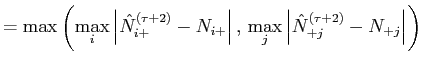
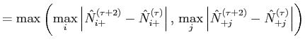
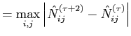
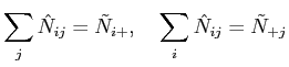
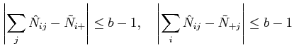
Using the termination criterion of Figure 2.4 (line 10), the IPF procedure will not necessarily terminate if two randomly rounded margins conflict. The termination criterion shown requires the fitted table to match all margins simultaneously:
 |
(20) |
 |
(21) |
 |
(22) |
For each cross-tabulation, statistical agencies publish a hierarchy
of margins, and these margins are rounded independently of the cells in the
table. For a three-way
table ![]() randomly rounded to give
randomly rounded to give
![]() ,
the data release will also include randomly rounded two-way margins
,
the data release will also include randomly rounded two-way margins
![]() ,
,
![]() and
and
![]() , one-way margins
, one-way margins
![]() ,
,
![]() and
and
![]() , and a zero-way
total
, and a zero-way
total
![]() . The sum of the cells does not necessarily match
the marginal total. For example, the sum
. The sum of the cells does not necessarily match
the marginal total. For example, the sum
![]() includes
includes
![]() randomly rounded counts. The expected value of this sum is the true
count
randomly rounded counts. The expected value of this sum is the true
count ![]() , but the variance is large and the sum could be off by as
much as
, but the variance is large and the sum could be off by as
much as ![]() in the worst case. By contrast, the reported marginal
total
in the worst case. By contrast, the reported marginal
total
![]() also has the correct expected value, but its
error is at most
also has the correct expected value, but its
error is at most ![]() .
.
For this reason, it seems sensible to include the hierarchical margins in the fitting procedure, in addition to the detailed cross-tabulation itself.
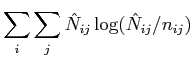
As described in equations (2.6)
and (2.1), the IPF procedure minimizes
the Kullback-Leibler divergence
![]() ,
,
 |
 |
That is, any value within the range
![]() is an
acceptable solution, with no preference for any single value within that
range.
is an
acceptable solution, with no preference for any single value within that
range.
Dykstra's generalization of IPF [17] provides some fruitful ideas for
handling this type of constraint. Csiszár [13] described the IPF
procedure as a series of projections onto the subspace defined by
each constraint. Csiszár was not working in a ![]() -dimensional space
(where
-dimensional space
(where ![]() is the number of attributes being fitted), but in a
is the number of attributes being fitted), but in a
![]() -dimensional space (where
-dimensional space (where ![]() is the number of cells in the
table) representing all possible probability distributions, which has since
been called
is the number of cells in the
table) representing all possible probability distributions, which has since
been called ![]() -space.
-space.
Nevertheless, the idea of projection is still useful: each iteration of IPF is a modification of the probability distribution to fit a margin. It is a “projection” in that it finds the “closest” probability distribution in terms of Kullback-Leibler divergence, just as the projection of a point onto a plane finds the closest point on the plane in terms of Euclidean distance. (Note, however, that Kullback-Leibler divergence is not a true distance metric.)
Csiszár only considered equality constraints. Dykstra extended
Csiszár's method to include a broader range of constraints: any closed
convex set in ![]() -space. This class of constraints appears to include the
desired inequality constraints defined by Equation 4.4.
Dykstra's method for applying these constraints is also a projection
procedure, finding the set of counts that satisfy the constraint while
minimizing the Kullback-Leibler divergence.
-space. This class of constraints appears to include the
desired inequality constraints defined by Equation 4.4.
Dykstra's method for applying these constraints is also a projection
procedure, finding the set of counts that satisfy the constraint while
minimizing the Kullback-Leibler divergence.
To give an example, consider the algorithm of Figure 2.4. Line 5 would be replaced with
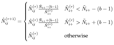 |
(24) |
|
However, this projection procedure has its own problems. The
standard IPF procedure ignores the probability distribution associated with
each marginal value and uses only the published cell count.
The projection procedure described here suffers from the opposite problem:
it focuses on the range of possible values, without acknowledging that
one outcome is known to be more likely than the others. To see this,
consider the probability distribution for the unrounded value ![]() given the published value
given the published value
![]() shown in
Table 4.4. The distribution is triangular, with a strong
central peak. The projection algorithm forces the fit to match the
range
shown in
Table 4.4. The distribution is triangular, with a strong
central peak. The projection algorithm forces the fit to match the
range ![]() of this distribution, but it treats all values inside
this range as equally probable. This would be suitable if the census used
unrestricted random rounding, but not for the more typical case where
unbiased rounding is used.
of this distribution, but it treats all values inside
this range as equally probable. This would be suitable if the census used
unrestricted random rounding, but not for the more typical case where
unbiased rounding is used.
Suppose that a population of person agents has been synthesized, with a limited amount of information about their relationships in families (such as a CFSTRUC, which classifies a person as married, a lone parent, a child living with parent(s), or a non-family person). In the absence of any information about how families form, the persons could be formed into families in a naïve manner: randomly select male married persons and attach them to female married persons, and randomly attach children to couples or lone parents. Immediately, problems would emerge: some persons would be associated in implausible manners, such as marriages with age differences over 50 years, marriages between persons living at opposite ends of the city, or parents who are younger than their children.
A well-designed relationship synthesis procedure should carefully avoid such problems. A good choice of relationships satisfies certain constraints between agents' attributes, such as the mother being older than her child, or the married couple living in the same zone. It also follows known probability distributions, so that marriages with age differences over 50 years have a low but non-zero incidence.
Most constraints and probability distributions are observed in microdata samples of aggregate agents, such as families and households. A complete Family PUMS includes the ages of mothers and children, and none of the records includes a mother who is younger than her children.3 Similarly, only a small fraction of the records include marriages between couples with ages differing by more than 50 years. The question, however, is one of method: how can relationships between agents be formed to ensure that the desired constraints are satisfied?
Guo & Bhat [26] used a top-down approach, synthesizing a household first and then synthesizing individuals to connect to the household. The attributes used to link the two universes were gender and age: the gender of the husband/wife or lone parent are known, and coarse constraints on the age of the household head (15-64 or 65+) and children (some 0-18 or all 18+). These constraints are quite loose, and no constraint is enforced between the husband/wife's ages or parent/child ages.
Guan [25] used a bottom-up approach to build families, with slightly stronger constraints. The persons were synthesized first, and then assembled to form families. Children are grouped together (and constrained to have similar ages), then attached to parents. Constraints between parent/child ages and husband/wife ages were included, although there are some drawbacks to the method used for enforcement. Guan likewise used a bottom-up approach to combine families and non-family persons into households.
Arentze & Timmermans [2] only synthesized a single type of agent, the household. Their synthesis included the age and labour force activity of both husband and wife, and the linkage to the number of children in the household. They did not connect this to a separate synthesis of persons with detailed individual attributes, but by synthesizing at an aggregate level, they guaranteed that the population was consistent and satisfied key constraints between family members.
Both Guo & Bhat and Guan's procedures suffer from inconsistencies between
the aggregate and disaggregate populations.
The family population may contain 50 husband-wife families in zone ![]() where
the husband has age
where
the husband has age ![]() , while the person population contains only 46
married males of age
, while the person population contains only 46
married males of age ![]() in zone
in zone ![]() . In the face of such
inconsistencies, either families or persons must be changed: a family
could be attached to a male of age
. In the face of such
inconsistencies, either families or persons must be changed: a family
could be attached to a male of age ![]() , or a person could be modified to
fit the family. In both cases, either the family or person population is deemed
“incorrect” and modified. The editing procedures are difficult to perform,
and inherently ad hoc. Furthermore, as the number of overlapping
attributes between the two populations grows, inconsistencies become
quite prevalent.
, or a person could be modified to
fit the family. In both cases, either the family or person population is deemed
“incorrect” and modified. The editing procedures are difficult to perform,
and inherently ad hoc. Furthermore, as the number of overlapping
attributes between the two populations grows, inconsistencies become
quite prevalent.
What are the sources of these inconsistencies? They come from two places:
first, the fitting procedure used to estimate the population distribution
![]() for persons and
for persons and
![]() for families may
not give the same totals for a given set of common attributes. Second, even if
for families may
not give the same totals for a given set of common attributes. Second, even if
![]() and
and
![]() agree on all shared
attributes, the populations produced by Monte Carlo synthesis may not
agree, since the Monte Carlo procedure is non-deterministic. In the
following sections, a method is proposed to resolve these two issues.
agree on all shared
attributes, the populations produced by Monte Carlo synthesis may not
agree, since the Monte Carlo procedure is non-deterministic. In the
following sections, a method is proposed to resolve these two issues.
For the purposes of discussion, consider a simple synthesis example:
synthesizing husband-wife families. Suppose that the universe of persons
includes all persons, with attributes for gender
![]() , family
status
, family
status
![]() , age
, age
![]() , education
, education
![]() and zone
and zone
![]() . The universe of families includes only
husband-wife couples, with attributes for the age of husband
. The universe of families includes only
husband-wife couples, with attributes for the age of husband
![]() and
wife
and
wife
![]() , and zone
, and zone
![]() . IPF has already been used
to estimate the contingency table cross-classifying persons
(
. IPF has already been used
to estimate the contingency table cross-classifying persons
(
![]() ) and likewise for the table of families
(
) and likewise for the table of families
(
![]() ). The shared attributes between the two
populations are age and zone, and implicitly gender. The two universes do
not overlap directly, since only a fraction of the persons belong
to husband-wife families; the others may be lone parents, children, or
non-family persons, and are categorized as such using the
). The shared attributes between the two
populations are age and zone, and implicitly gender. The two universes do
not overlap directly, since only a fraction of the persons belong
to husband-wife families; the others may be lone parents, children, or
non-family persons, and are categorized as such using the
![]() attribute.
attribute.
In order for consistency between
![]() and
and
![]() , the following must be met for
, the following must be met for
![]() and any choice of
and any choice of ![]() :
:
That is, the number of married males of age ![]() in zone
in zone ![]() must be the
same as the number of husband-wife families with husband of age
must be the
same as the number of husband-wife families with husband of age ![]() in zone
in zone
![]() . While this might appear simple, it is often not possible with the
available data. A margin
. While this might appear simple, it is often not possible with the
available data. A margin
![]() giving the
giving the
![]() distribution is probably available to apply to
the person population. However, a similar margin for just married males
is not likely to exist for the family population; instead, the age
breakdown for married males in the family usually comes from the PUMS
alone. As a result, equation (4.6) is not satisfied.
distribution is probably available to apply to
the person population. However, a similar margin for just married males
is not likely to exist for the family population; instead, the age
breakdown for married males in the family usually comes from the PUMS
alone. As a result, equation (4.6) is not satisfied.
One suggestion immediately leaps to mind: if the person population is
fitted with IPF first and
![]() is known,
the slice of
is known,
the slice of
![]() where
where
![]() and
and
![]() could be applied as a margin to the family
fitting procedure, and likewise for
could be applied as a margin to the family
fitting procedure, and likewise for
![]() . This is entirely
feasible, and does indeed guarantee matching totals between the
populations. The approach can be used for the full set of attributes shared
between the individual and family populations. There is one downside,
however: it can only be performed in one direction. The family table can be
fitted to the person table or vice versa, but they cannot be fitted
simultaneously.4
. This is entirely
feasible, and does indeed guarantee matching totals between the
populations. The approach can be used for the full set of attributes shared
between the individual and family populations. There is one downside,
however: it can only be performed in one direction. The family table can be
fitted to the person table or vice versa, but they cannot be fitted
simultaneously.4
Finally, there remains one wrinkle: it is possible that the family population will still not be able to fit the total margin from the individual population, due to a different sparsity pattern. For example, if the family PUMS includes no families where the male is (say) 15-19 years old but the individual PUMS does include a married male of that age, then the fit cannot be achieved. This is rarely an issue when a small number of attributes are shared, but when a large number of attributes are shared between the two populations it is readily observed. The simplest solution is to minimize the number of shared attributes, or to use a coarse categorization for the purposes of linking the two sets of attributes.
Alternatively, the two PUMS could be cross-classified using the shared
attributes and forced to agree. For example, for
![]() and
and
![]() , then the pattern of zeros in
, then the pattern of zeros in
![]() and
and
![]() could be forced to agree by
setting cells to zero in one or both tables. (In the earlier example, this
would remove the married male of age 15-19 from the Person PUMS.) The person
population is then fitted using this modified PUMS, and the family
population is then fitted to the margin of the person population.
could be forced to agree by
setting cells to zero in one or both tables. (In the earlier example, this
would remove the married male of age 15-19 from the Person PUMS.) The person
population is then fitted using this modified PUMS, and the family
population is then fitted to the margin of the person population.
The second problem with IPF-based synthesis stems from the independent
Monte Carlo draws used to synthesize persons and families. For example,
suppose that mutually fitted tables
![]() and
and
![]() are used with Monte Carlo to produce a complete
population of persons and families
are used with Monte Carlo to produce a complete
population of persons and families
 and
and
 . If it can be guaranteed for
![]() and
and
![]() that
that
A simplistic solution would be a stratified sampling scheme: for each
combination of ![]() and
and ![]() , select a number of individuals to synthesize
and make exactly that many draws from the subtables
, select a number of individuals to synthesize
and make exactly that many draws from the subtables
![]() and
and
![]() . This approach
breaks down when the number of strata grows large, as it inevitably does
when more than one attribute is shared between persons and families.
. This approach
breaks down when the number of strata grows large, as it inevitably does
when more than one attribute is shared between persons and families.
The problem becomes clearer once the reason for mismatches is recognized.
Suppose a Monte Carlo draw selects a family with husband age ![]() in
zone
in
zone ![]() . This random draw is not synchronized with the draws from the
person population, requiring a person of age
. This random draw is not synchronized with the draws from the
person population, requiring a person of age ![]() in zone
in zone ![]() to be drawn;
the two draws are independent. Instead, synchronization could be achieved
by conditioning the person population draws on the family population
draws. Instead of selecting a random value from the joint
distribution
to be drawn;
the two draws are independent. Instead, synchronization could be achieved
by conditioning the person population draws on the family population
draws. Instead of selecting a random value from the joint
distribution
This reversal of the problem guarantees that equation (4.7) is satisfied, and allows consistent relationships to be built between agents. While it has been described here in a top-down manner (from family to person), it can be applied in either direction. The two approaches are contrasted in Figures 4.2 and 4.3.
As demonstrated in the preceding sections, it is possible to synthesize
persons and relate them together to form families, while still guaranteeing
that the resulting populations of persons and families approximately
satisfy the fitted tables
![]() and
and
![]() . By
carefully choosing a set of shared attributes between the person and
family agents and using conditional synthesis, a limited number of
constraints can be applied to the relationship formation process. In the
example discussed earlier, the ages of husband/wife were constrained; in a
more realistic example, the labour force activity of husband/wife, the
number of children and the ages of children might also be constrained.
Furthermore, multiple levels of agent aggregation could be defined: families
and persons could be further grouped into households and attached to
dwelling units.
. By
carefully choosing a set of shared attributes between the person and
family agents and using conditional synthesis, a limited number of
constraints can be applied to the relationship formation process. In the
example discussed earlier, the ages of husband/wife were constrained; in a
more realistic example, the labour force activity of husband/wife, the
number of children and the ages of children might also be constrained.
Furthermore, multiple levels of agent aggregation could be defined: families
and persons could be further grouped into households and attached to
dwelling units.
The synthesis order for the different levels of aggregation can be varied as required, using either a top-down or bottom-up approach. However, the method is still limited in the types of relationships it can synthesize: it can only represent nesting relationships. Each individual person can only belong to one family, which belongs to one household. Other types of relationships cannot be synthesized using this method, such as a person's membership in another group (e.g., a job with an employer).


![\begin{algorithm}
% latex2html id marker 3311
[p]\For{$1 \ldots N^F$}{
Synthe...
...n algorithm for synthesizing persons and husband-wife
families.}
\end{algorithm}](img290.png)
![\begin{algorithm}
% latex2html id marker 3320
[p]\For{$1 \ldots N^P$}{
Synthe...
...p algorithm for synthesizing persons and husband-wife
families.}
\end{algorithm}](img291.png)