| [PDF] |
|
| [PDF] |
|
It is challenging to evaluate the results of a data synthesis procedure. If any form of complete “ground truth” were known, the synthetic population could be tested for goodness-of-fit against the true population's characteristics; but instead only partial views of truth are available in smaller, four-way tables.
In theory, IPF-based procedures have many of the qualities necessary for a good synthesis: an exact fit to their margins, while minimizing the changes to the PUMS (using the discrimination information criterion). This does not mean that the full synthesis procedure is ideal: the fit may be harmed by conflicting margins (due to random rounding), and will almost certainly be poorer after Monte Carlo (or conditional Monte Carlo). Furthermore, it still leaves a major question open: how much data is sufficient for a “good” synthesis? Are the PUMS and multidimensional margins both necessary, or could a good population be constructed with one of these two types of data? Does the multizone method offer a significant improvement over the zone-by-zone approach?
To answer these questions, a series of experiments was conducted. In the absence of ground truth, each synthetic population is evaluated in terms of its goodness-of-fit to a large collection of low-dimensional contingency tables. These validation tables are divided into the following groups:
After cross-classifying the synthetic population to form one table
![]() , it can be compared to a validation table
, it can be compared to a validation table
![]() using various goodness-of-fit statistics. This is
repeated for each of the validation tables in turn, and the goodness-of-fit
statistics in each group are then averaged together to give an overall
goodness-of-fit for that group.
using various goodness-of-fit statistics. This is
repeated for each of the validation tables in turn, and the goodness-of-fit
statistics in each group are then averaged together to give an overall
goodness-of-fit for that group.
The choice of evaluation statistic is challenging, with many trade-offs.
Knudsen & Fotheringham provided a good and even-handed overview of
different matrix comparison statistics [31], framed in the
context of models of spatial flows, but applicable to many other matrix
comparison problems. They reviewed three categories of statistics:
information theoretic, generalized distance, and traditional statistics
(such as ![]() and
and ![]() ). In a comparison of the statistics, their
ideal was “one for which the relationship between the value of the
statistic and the level of error is linear,” and using this benchmark they
found that the Standardized Root Mean Square Error (SRMSE) and
). In a comparison of the statistics, their
ideal was “one for which the relationship between the value of the
statistic and the level of error is linear,” and using this benchmark they
found that the Standardized Root Mean Square Error (SRMSE) and
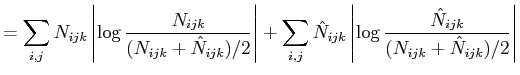
![]() were the “best” statistics. The former is a representative
distance-based statistic, while the latter is an unusual information
theoretic statistic. As Voas & Williamson noted,
were the “best” statistics. The former is a representative
distance-based statistic, while the latter is an unusual information
theoretic statistic. As Voas & Williamson noted,
![]() is actually
very little different from another distance-based statistic, total absolute
error [53].
is actually
very little different from another distance-based statistic, total absolute
error [53].
| SRMSE | 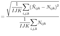 |
(28) |
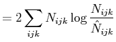
 |
(29) |
 |
An example comparing the two types of statistics is shown in
Table 6.1. In the experiment shown, the population was
fitted using a zone-by-zone method, with all available Summary Tables
applied as margins (identical to experiment I8 in the following section).
A good fit is expected in the first four groups of validation tables, and a
reasonable fit is expected for the final group since the initial table
was the complete PUMS. In terms of fit, the SRMSE statistic matches
expectations. In terms of information, the ![]() statistic shows a huge
improvement over a null model; in other words, most of the information
present in the tables is explained by the fitted population. However, using
the
statistic shows a huge
improvement over a null model; in other words, most of the information
present in the tables is explained by the fitted population. However, using
the ![]() statistic, the poorest group of validation tables
is not group five but group four (2-3D STs by zone); these tables
are where most of the missing information lies.
statistic, the poorest group of validation tables
is not group five but group four (2-3D STs by zone); these tables
are where most of the missing information lies.
Nevertheless, distance-based statistics are more widespread in the literature, and have been reported for many other population synthesis applications. For these reasons, the SRMSE statistic is used as the primary evaluation metric here. It is scaled by 1000 throughout, rather than 100,000 as above.
Finally, it would be useful to also be able to apply traditional statistical tests to compare different models. In particular, tests such as the Akaike Information Criterion (AIC) which reward parsimonious low-parameter models would be interesting to apply. However, because the data is sparse, it is difficult to determine the number of degrees of freedom and the number of free parameters during Iterative Proportional Fitting. Without this information, statistical tests are not possible.
| |||||||||||||||||||||||||||||||||||||||||||||||||||||||||||||||||||||||||||||||||||||||||||||||||||||||||||||||||||||||||||||||||||||||||||||||||||||||||||||||||||||||||||||||||||||||||||||||||||||||||||||||||||||||||||||
In the first series of experiments, the IPF procedure is tested with different inputs to see how the quality of fit is affected. Three questions are tested simultaneously:
To test these hypotheses, a set of ten fits was conducted, labelled I1 through I10. Essentially, the experiments evaluate these three different questions, showing the impact of different source samples, 1D versus 2-3D margins, and three different approaches to geography. The input data included in each experiment are shown together with the output goodness-of-fit in Table 6.2. The first set of experiments (I1-I4) show the results with no geographic input data, and are largely intended as a “base case” to show the effect of better data. Experiments I5-I8 show a zone-by-zone IPF method, where each zone is fitted independent of the others. I6 represents a “typical” application of IPF for population synthesis: a zone-by-zone approach using 1D margins. Finally, I9 and I10 show the multizone approach suggested by Beckman et al., where the PUMS is applied as a marginal constraint.
The combinatorial optimization method is not IPF-based, but it does operate on a zone-by-zone basis. It is not possible to determine which of the experiments I5-I8 is “closest” to combinatorial optimization. While combinatorial optimization starts with a random sample of the PUMS, it does not guarantee that the final result fits the PUMS associations (validation table group 5); it almost certainly has a poorer fit to group 5 than I6 or I8. Furthermore, the method does have some convergence issues when applying a large number of constraints, and it is not clear whether the full set of 2-3D constraints could be applied in a practical implementation. As a result, the combinatorial optimization method might give a fit close to any of I5-I8, or possibly even poorer than I5; without a direct comparison, little can be said.
To evaluate the effect of source sample, compare the use of a constant initial table filled with ones (I1, I3, I5 and I7) to the use of the PUMS as the initial table (I2, I4, I6 and I8).7 Because a sparse IPF procedure is used, the initial table necessarily has the sparsity pattern of the PUMS in all cases. The constant initial table's non-zero cells were all ones, while the PUMS initial table initially had many higher integer cells.
In all cases, the use of the PUMS for the initial table drastically improves the fit to validation group 5 (2-3D PUMS-only) by at least an order of magnitude. In experiments I2 and I6 where no 2-3D margins are applied, the use of PUMS similarly improves the fit to validation group 3 (2-3D STs, entire PUMA). However, the improvement is considerably smaller on validation group 4 (2-3D STs by zone).
All of these are expected results. The only interesting finding is for I6: there are geographical variations in the 2-3D association pattern that are not explained by the combination of 1D margins with geography and the PUMS.
To observe the effect of higher-dimensional margins, compare the experiments with 1D margins (I1, I2, I5, I6, I9) against the experiments with 2-3D margins (all others). From a brief glance at the results, it is quickly evident that there is multiway variation in the data that is not explained unless either the PUMS or 2-3D margins are applied. For validation groups 1 and 3 (1D and 2-3D STs, entire PUMA), the difference between inputting the PUMS (I2, I6, I9) or the 2-3D margins (I3, I7, I10) is fairly small. The main difference is due to sample size: the PUMS is a 2% sample, while the margins are drawn from 20% samples.
The primary benefit of including 2-3D margins appears to be the ability to capture geographic variation in these 2-3 way relationships. The goodness-of-fit against these validation tables remains poor until the 2-3D Summary Tables by zone are included in I7, I8 and I10.
The difference between the zone-by-zone and multizone methods was surprisingly small. While the zone-by-zone method makes no attempt to explicitly fit validation groups 1 and 3 (1D and 2-3D STs, entire PUMA), it still seems to achieve a fairly good fit.
The only improvement recorded by the multizone method is in the fit to validation group 5 (2-3D, PUMS only): I9 does better than I6 on this score, and I10 likewise does better than I8. Nevertheless, the difference is fairly small.
The reasons for the difference lie in the contrasting approaches to the PUMS. In many cases, the fit to the initial table decreases as more margins are included in the IPF. The additional margins show up as more terms in the log-linear model and appear as additional free parameters during the fitting process, giving the fitted table more freedom to vary from the source table. Deterioration of fit to the source table can be clearly seen by comparing I2 to I6 or I4 to I8. The I6 experiment added new tables with geographic variation; however, this does not improve the fit to the PUMA-wide 2-3D PUMS-only tables (validation group 5). Indeed, the fit to these tables deteriorates due to the addition of parameters.
By contrast, the multizone approach forces a fit to the PUMS, treating it as a margin with equal importance to the other constraints. As a result, it achieves a better fit to validation group 5.
| |||||||||||||||||||||||||||||||||||||||||||||||||||||||
In a second series of experiments, the effects of random rounding were tested. Table 6.3 shows the results of four experiments. The first two (R1 and R2) show the effects of hierarchical margins when using a zone-by-zone algorithm, and the second two (R3 and R4) show the effects when using a multizone algorithm.
As shown, there is a small improvement in fit when using hierarchical margins. The improvement of fit at the zonal level is somewhat surprising—after all, when hierarchy is not used, the only input margins are the zonal tables. However, the improvement comes due to conflicts between tables sharing the same attributes. In R1 and R3, the fit to the final zonal table is perfect, but the other zonal tables have a poorer fit than in R2 and R4.
Overall, this suggests that hierarchical margins are useful, but their impact on goodness-of-fit is relatively small.
| ||||||||||||||||||||||||||||||||||||||||||||
In a third series of experiments, the effects of the Monte Carlo integerization procedures are tested. The design and results of these experiments are shown in Table 6.4. The first experiment M0 is the null case: the results of the IPF procedure before any Monte Carlo integerization takes place. Experiment M1 shows the conventional Monte Carlo procedure, where a set of persons are synthesized directly from the IPF-fitted tabulation for persons. Experiment M2 is the conditioned Monte Carlo procedure described in Chapter 5, where households/dwellings are synthesized by Monte Carlo, families are conditionally synthesized on dwellings, and persons are conditionally synthesized on families. The results are evaluated on the person population only, to focus on the effects of the two stages of conditioning prior to generating the persons.
As expected, the goodness-of-fit deteriorates after applying Monte Carlo, and deteriorates further using the conditional procedure. The deterioration from M0 to M1 is somewhat larger than the deterioration from M1 to M2. In essence, this shows that the conditional synthesis procedure employed here does not have a major impact on the goodness-of-fit. Even after two stages of conditioning (from dwellings to families to persons), a reasonable goodness-of-fit is maintained.
Additionally, among the tables in validation group 1 (1D STs, entire PUMA) in Table 6.4, there is one clear outlier: the fit to CTCODE had an average SRMSE × 1000 of 16 for M1 and 30 for M2. This poor fit—and the poorer fits to validation group 2 (1D STs, by zone)—might be corrected by stratifying the Monte Carlo synthesis by zone, although this could cause a deterioration of the fits to the non-geographic tables.