| [PDF] |
|
| [PDF] |
|
The data for this project came largely from the Canadian Census administered by Statistics Canada. The census has been conducted every five years since 1981, and Toronto's travel activity survey (the Transportation Tomorrow Survey or TTS) is timed to coincide with census years. The TTS was first conducted in 1986, and this was therefore chosen as the baseline year for the ILUTE model and population synthesis.
The Canadian Census has been conducted as a mail-back self-administered survey since 1971. Eighty percent of households receive a short survey known as the 2A form, while twenty percent receive an expanded version called the 2B form. In 1986, the census was conducted on the first Tuesday of June, which fell on the third day of the month. The 1986 Census was Canada's first full mid-decade census, and was very nearly cancelled due to reduced federal government expenditure in the early 1980s. It was reinstated, but with limited resources. As a result, some useful information was never fully coded or tabulated, such as the place-of-work. However, the provincial government in Ontario did pay for geocoding place-of-work for the entire province, and some tables with geographic distributions of employment do exist, although they can be difficult to obtain [47].
Census data is aggregated by persons, census families, or households and is released in three distinct forms. Profile tables are assembled for each question from the census, showing the breakdown of responses to a single question within a geographic area. Basic Summary Tabulations (BSTs) are cross-tabulations of two to four questions from the census, also including geographic variation. Profile table and cross-tabulations may be derived from questions from the 2A or 2B forms, and may represent either a 100% sample or a 20% sample that has been expanded to a 100% basis. Finally, Statistics Canada also releases Public Use Microdata (PUMS), a 2% sample of all responses made by a person (and likewise a 1% sample of family responses and a 1-4% sample of household responses). Each PUMS data file is associated with a single Census Metropolitan Area (CMA), a large geographic area of more than 100,000 persons that acts as the equivalent of the Public Use Micro Area (PUMA) in the U.S.; the data contains no information about spatial variation within the CMA.
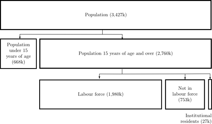 |
The PUMS data and different summary tables may be drawn from different samples. The population of persons can be broken down into many subgroups, some of which are shown in Figure 3.1. The 2A census form (100% sample) is collected for the full population, while the 2B form (20% sample) is collected only for the non-institutional population 15 years of age and over. Some summary tables are defined on the 2A universe, where exact population counts are available. Others are defined on the 2B universe, by expanding the 20% sample to an estimate of the complete 2B universe. Combining data from tables derived from the 2A and 2B samples can be challenging, because of their differing universes and errors in the 2B estimates. The PUMS uses a different sample again; it is defined on a 2% sample of the full population excluding institutional residents (and residents of incompletely enumerated Indian reserves, which are not an issue in the Toronto CMA). The sample sizes associated with different universes and tables are summarized in Table 3.1.
The universe of persons is slightly complicated. The 1986 census excluded non-permanent residents from all tables, which includes foreign persons present on student authorization, employment authorization, Minister's permits and refugee claimants. These were included in 1991 and subsequent censuses, and do account for a sizeable fraction of the Toronto population. In 1991, there were 98,105 non-permanent residents in the Toronto CMA (2.5% of total); assuming a similar growth rate to the CMA as a whole, this would give approximately 89,000 in 1986. There is no data on this population, however. Institutional collective dwellings are defined as hospitals, orphanages, correctional/penal institutions and religious institutions, and the residents of these institutions are excluded from many tables (but not the staff). Non-institutional collective dwellings are defined as hotels, motels, tourist homes, lodging- and rooming-houses, work camps, military camps and Hutterite colonies. Temporary residents are persons with a usual dwelling elsewhere in Canada living temporarily in another dwelling; they are usually treated as part of their “permanent” household. However, some dwellings are occupied only by temporary residents, and are a separate category from both occupied and unoccupied dwellings. Finally, foreign residents are foreign diplomats or military personnel stationed in Canada. Temporary, foreign and collective (non-institutional) residents are included in most person-based tables, but not in family, household or dwelling tables.
Statistics Canada makes some modifications to the collected census data
before publishing tables. Contradictions in the submitted form are
resolved using an edit and impute method.
Furthermore, to protect the privacy of individual persons and households,
Statistics Canada applies two disclosure control techniques. In any
released table, all numbers are randomly rounded (up or down) to
a multiple of five and in special cases to a multiple of ten. This is a
stronger measure than many countries; the UK and New Zealand use a multiple
of three, and the American census does not use random rounding [18].
The UK and Australian agencies apply random rounding only to small cells, but
the Canadian agency applies it to every cell in every table. In each
reported table, the individual cells and the row and column totals are
rounded independently using a procedure called Unbiased Random Rounding.
The rounding tends toward the closer multiple of five, so a count of 4
has a probability of 80% of being rounded to 5 and a 20% probability of
being rounded to 0 [55]. The alternative is called unrestricted random rounding, where there is a fixed probability ![]() that
a cell is rounded down, regardless of its value; typically,
that
a cell is rounded down, regardless of its value; typically, ![]() is
used.1
is
used.1
Finally, in geographic areas with less than forty persons, no data is released; this is called area suppression. Additionally, in areas with less than 250 persons, no income data is released.
The Canadian census family and household definitions are generally intuitive, but some special cases are tricky. As the Census Handbook notes, “it is very difficult to translate complex human relationships into tables” [42].
|
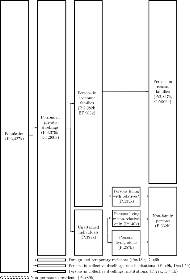
The census distinguishes between two types of families: the “census family” defines a relationship between cohabiting adults and children, while the “economic family” defines other types of family relationships within a single dwelling. The details of family definition are complicated, particularly when considering cohabiting multigeneration families. The household definition is straightforward, consisting of all persons sharing a “dwelling unit;” there is a one-to-one relationship between households and occupied dwelling units. The dwelling unit definition is slightly more complicated, and is defined as living quarters with a private entrance from the outside or from a common hallway. More formally, Figure 3.2 graphically shows the relationship between the different types of family membership.
“People living in the same dwelling are considered a census family only if they meet the following conditions: they are spouses or common-law partners, with or without never-married sons or daughters at home, or a lone parent with at least one son or daughter who has never been married. The census family includes all blood, step- or adopted sons and daughters who live in the dwelling and have never married. It is possible for two census families to live in the same dwelling; they may or may not be related to each other” [49] for 1996; essentially the same as 1986 definition [42,45].
No distinction is made between common-law and legal marriage; both are coded as “married.” While homosexual couples are recognized to exist, the census coding does not allow this type of family. Any household that reports a married/common-law couple with the same sex is recoded; either they are cohabiting unmarried individuals or the gender of one individual is changed, making it an opposite-sex marriage [45]. Finally, foster children are treated as lodgers rather than family members. Table 3.2 details an example household that illustrates several unusual aspects of these family definitions.
|
The connection between households and families is also illustrated in Figure 3.2. Each “private household” occupies one dwelling, in the language of the census. This one-to-one relationship between private households and “occupied private dwellings” means that the household PUMS can be used as a PUMS for dwellings. Occupied private dwellings are only one part of the dwelling universe, but almost no data is available on other types of dwellings. The missing parts of this universe are collective dwellings, dwellings occupied by foreign/temporary residents, unoccupied dwellings, some marginal dwellings (e.g., cottages that are not occupied year-round), and some dwellings under construction or conversion.2
| ||||||||||||||||||||||||||||||||||||||||||||||||||||||||||||||||||||||||||||||||||||||||||||||||||||||||||||||||||||||||
| |||||||||||||||||||||||||||||||||||||||||||||||||||||||||||||||||||||||||||||||||||||||||||||||||||||||||||||||||||||||||||||||||||||||||||||||||||||||||||
| ||||||||||||||||||||||||||||||||||||||||||||||||||||||||||||||||||||||||||||||||||||||||||||||||||||||||||||||||||||||||||||||||||||||||||||||||||||||||||
The census offers a broad range of attributes that could be used in synthesis. Tables 3.3, 3.4 and 3.5 show the attributes selected for synthesis, and the relevant data sources that include these attributes.
Both the Household PUMS and the Family PUMS lack information on the number of census families sharing a dwelling, and the Family PUMS also lacks information about the household size. These attributes would be useful, but can fortunately be derived from another source: the Person PUMS. Suppose that we consider only the family persons in the Person PUMS, and treat each person as an observation of a census family. Then, the attributes from the Person PUMS could be used to derive information about census families. A similar procedure could be used to gain additional information about households.
However, persons in large families are over-represented in the person PUMS.
For example, consider the complete population of families and persons,
ignoring for the moment the small sample in the PUMS itself. A family of
eight persons is repeated eight times in the person population, while a
family of two persons is repeated twice. Large families are thus
overrepresented in the person population, but this can be corrected by
weighting each observation in the person population by
![]() , the
inverse of the family size. In the PUMS, not every member of an eight-person
family will be present in the Person PUMS, but large families will still be
observed proportionately more often, and the same reweighting method can be
applied to correct this.
, the
inverse of the family size. In the PUMS, not every member of an eight-person
family will be present in the Person PUMS, but large families will still be
observed proportionately more often, and the same reweighting method can be
applied to correct this.
| ||||||||||||||||||||||||||||||||||||||||||||||||||||||||||||||||||||||||||||||||||||||||||||||||||||||||||||||||
|
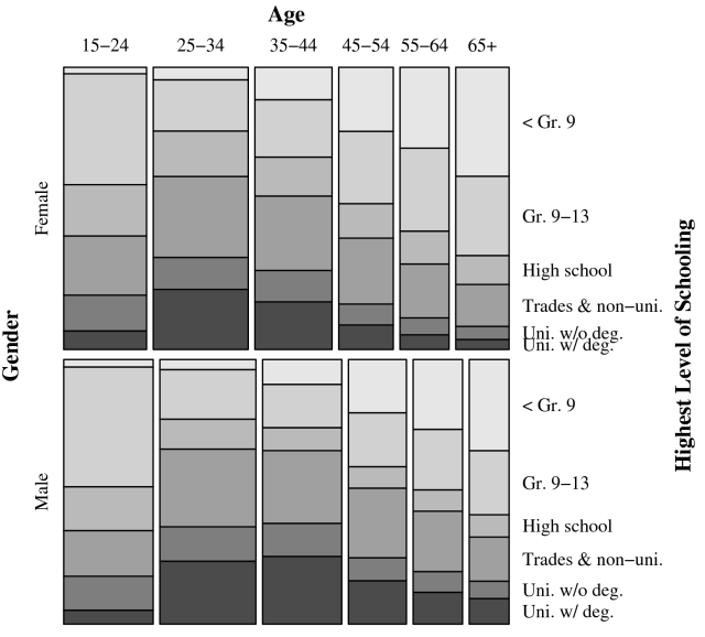
To help understand the census data (and contingency tables in general), a brief examination of a single summary table is useful. This exploration focuses on the SC86B01 table, a summary table that cross-classifies age, sex and education by zone. The study area is the Toronto CMA, and the geography has been simplified to a set of twelve zones. Table 3.6 shows the counts in SC86B01, excluding the geographic breakdown. Figure 3.3 shows the same information graphically.
What are the statistical properties of this table? Is there statistically
significant association between these variables? Is there significant
geographic variation? A log-linear model can be used to answer these
questions. In the following, the variables ![]() ,
, ![]() ,
, ![]() and
and ![]() will be used to represent gender, age, level of schooling and zone respectively.
will be used to represent gender, age, level of schooling and zone respectively.
First, to consider statistically significant association between the variables
(excluding geography), a hierarchy of models can be constructed. The
final model in this hierarchy
![]() defines all-way association
between the non-geographic variables, and is given by
defines all-way association
between the non-geographic variables, and is given by
| (18) |
|
To test for this three-way association, the ![]() statistics of model
statistics of model
![]() and the restricted model
and the restricted model
![]() are compared and tested
using a chi-squared distribution. Because SC86B01 is derived from a 20% sample that was expanded to 100%, the
counts must be deflated by a factor of five before estimating the models.
Table 3.8 shows the complete series of models leading up
to
are compared and tested
using a chi-squared distribution. Because SC86B01 is derived from a 20% sample that was expanded to 100%, the
counts must be deflated by a factor of five before estimating the models.
Table 3.8 shows the complete series of models leading up
to
![]() . Each model in the series exhibits statistically significant
improvement in fit over the previous model. Consequently, we can reject the
hypothesis that there is no three-way association between gender, age and
highest level of schooling.
. Each model in the series exhibits statistically significant
improvement in fit over the previous model. Consequently, we can reject the
hypothesis that there is no three-way association between gender, age and
highest level of schooling.
|
In a second series of models, the influence of geography is included.
(In this analysis, the simplified 12-zone representation of geography is
used; the full 731-zone system cannot be analyzed with a log-linear model,
due to the memory requirements of generalized linear model estimation.)
Table 3.8 shows the series of log-linear models
leading up to the saturated model
![]() . As shown, every model is
statistically significant with respect to the next
simplest model; we can therefore conclude that there is significant
four-way association in this dataset. Furthermore, the
. As shown, every model is
statistically significant with respect to the next
simplest model; we can therefore conclude that there is significant
four-way association in this dataset. Furthermore, the
![]() model describes 95% of the deviance in the data; while the
higher-order geographic associations are statistically significant,
they are responsible for only a small part of the total deviance.
model describes 95% of the deviance in the data; while the
higher-order geographic associations are statistically significant,
they are responsible for only a small part of the total deviance.
|
The final set of models shown in Table 3.9
simulate the effect of using IPF with a particular set of margins from
SC86B01. The left hand side follows equation (2.18),
dividing the fitted margins of SC86B01 (
![]() ) by the PUMS
(
) by the PUMS
(![]() ):
):
| (19) |
Furthermore, the inclusion of higher-order interactions shows
diminishing returns in terms of the explained deviance. The one-way
model ![]() explains 92.3% of the deviance in the NULL model.
Of the remaining 7.7% of total deviance, the two-way model
explains 92.3% of the deviance in the NULL model.
Of the remaining 7.7% of total deviance, the two-way model
![]() explains 86.6%. Of the final 1.0% of total
deviance, the three-way model
explains 86.6%. Of the final 1.0% of total
deviance, the three-way model
![]() explains 89.2% and the
four-way model
explains 89.2% and the
four-way model
![]() explains the final 10.8%.
The total deviance does depend on the choice of variables and the fineness of
the categories in the table, but this trend of diminishing
returns is interesting. It suggests that the available census
data—largely describing lower-order interactions, with only a few
higher-order interactions, apart from the 2%-sample PUMS—may capture the
bulk of the actual information about the population. However, this single
table is clearly not sufficient to say anything conclusive.
explains the final 10.8%.
The total deviance does depend on the choice of variables and the fineness of
the categories in the table, but this trend of diminishing
returns is interesting. It suggests that the available census
data—largely describing lower-order interactions, with only a few
higher-order interactions, apart from the 2%-sample PUMS—may capture the
bulk of the actual information about the population. However, this single
table is clearly not sufficient to say anything conclusive.
In closing, this analysis has focused on a single contingency table, SC86B01. No attempt was made to find the best model for SC86B01, particularly in terms of model parsimony; instead, the analysis demonstrated that statistically significant higher-order interactions are present in the data. Furthermore, it is not possible to apply this type of log-linear analysis to multiple contingency tables, although if multiple tables are combined using a fitting procedure the result could be analyzed. The largest limitation, however, is one of software: log-linear analysis is not generally feasible with high-dimensional tables. Nevertheless, the analysis provides valuable insight about the utility of information recorded in contingency tables.