| [PDF] |
|
| [PDF] |
|
The research described in this thesis draws on a broad body of knowledge. This literature review begins with a section on the context for this population synthesis effort, the Integrated Land Use Transportation, Environment (ILUTE) model.
The following section describes the mathematics and algorithms used in population synthesis, starting with a discussion of notation for contingency tables. The properties and history of the Iterative Proportional Fitting (IPF) procedure are reviewed, and some generalizations of the method are discussed in the following section. The discussion then shifts to log-linear modelling for contingency tables, and then looks briefly at the literature connecting IPF and log-linear modelling. The final section reviews the literature dealing with zeros in contingency tables.
The review then shifts to the methods used for population synthesis. Two broad classes of method are included: those using IPF and those using the Combinatorial Optimization method.
|
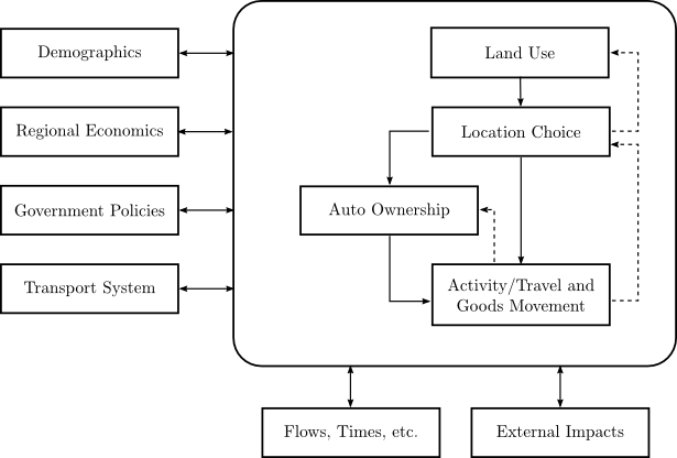
The ILUTE research program aims to develop next generation models of urban land use, travel and environmental impacts. The project's ultimate goal is the “ideal model” described by Miller et al. [34]. As shown in Figure 2.1, the behavioural core of an ideal model would include land development, residential and business location decision, activity/travel patterns and automobile ownership. The boxes on the left show the main influences on the urban system: demographic shifts in the population, the regional economy, government policy and the transport system itself. Some of these may be exogenous inputs to the model, but Miller et al. suggest that both demographics and regional economics need to be at least partially endogenous.
The ILUTE model is intended to operate in concert with an activity-based travel demand model. The Travel/Activity Scheduler for Household Agents (TASHA) is an activity-based model designed on disaggregate principles similar to ILUTE, and connects personal decision making with household-level resources and activities to form travel chains and tours [35,36].
The operational prototype of the ILUTE system was described in detail by Salvini & Miller [40,39]. To validate the model, it is intended to be run using historical data, allowing comparison against the known behaviour of the urban system over recent years. The baseline year of 1986 was ultimately chosen as a starting point, since the Transportation Tomorrow Survey of travel behaviour in the Greater Toronto Area was first conducted in that year.
The prototype defines a wide range of agents and objects: persons, households, dwellings, buildings, business establishments and vehicles. It also defines various relationships between these agents and objects: in particular, family relationships between persons in households, occupancy relationships between households and their dwellings, ownership of dwellings/vehicles by households or persons, containment of dwellings within buildings, and employment of persons by business establishments.
These represent the full spectrum of possible agents and relationships that need to be synthesized as inputs to the ILUTE model. In earlier work within the ILUTE framework, Guan synthesized persons, families and households and a set of relationships between them [25]. In this thesis, the same agents and relationships are considered (in addition to dwelling units), with the goal of improving the method and quality of the synthetic populations.
The remaining agents and relationships are also important to the ILUTE model, but the focus here is on the demographic and dwelling attributes since these are central to both the ILUTE and TASHA models, and because rich data from the Canadian census is available to support the synthesis. In this research, families are proposed as a new class of agent for the ILUTE modelling framework. While the family is a central theme in both the ILUTE and TASHA models, it was only modelled distinct from the household in Guan's work. Furthermore, the original ILUTE prototype did not allow for multifamily households.
Almost all population synthesis procedures rely on data stored in multiway contingency tables. To help understand and explain this type of data, a consistent notation is first defined, and then the mathematical properties of contingency tables and the Iterative Proportional Fitting procedure are described.
Throughout this document, scalar values and single cells in contingency
tables will be represented using a regular weight typeface (e.g., ![]() or
or
![]() ). Multiway contingency tables and their margins will be represented
with boldface (e.g.,
). Multiway contingency tables and their margins will be represented
with boldface (e.g.,
![]() or
or
![]() ) to indicate that they
contain more than one cell. Contingency tables may be one-way, two-way or
multiway; the number of subscripts indicates the dimension of the table
(e.g.,
) to indicate that they
contain more than one cell. Contingency tables may be one-way, two-way or
multiway; the number of subscripts indicates the dimension of the table
(e.g.,
![]() ).
).
Suppose three variables ![]() ,
, ![]() and
and ![]() vary simultaneously, and are classified
into
vary simultaneously, and are classified
into ![]() ,
, ![]() and
and ![]() categories respectively. The variables may be either
inherently discrete or continuous, but continuous variables are grouped into a
finite set of discrete categories. The variable
categories respectively. The variables may be either
inherently discrete or continuous, but continuous variables are grouped into a
finite set of discrete categories. The variable ![]() denotes a category of
denotes a category of
![]() , and the categories are labelled as
, and the categories are labelled as
![]() , and likewise
for
, and likewise
for ![]() and
and ![]() . (For example, suppose that these variables represent
the attributes of a person, such as age, education and location.) Then, there
is a probability
. (For example, suppose that these variables represent
the attributes of a person, such as age, education and location.) Then, there
is a probability ![]() that a random observation will be classified in
category
that a random observation will be classified in
category ![]() of the first variable, category
of the first variable, category ![]() of the second variable and
category
of the second variable and
category ![]() of the third variable. There are
of the third variable. There are
![]() cells in
the table, each of which consists of a count
cells in
the table, each of which consists of a count ![]() of the number of
observations with the appropriate categories. Since the table consists of
counts, the cells are Poisson distributed; these counts are observations of
the underlying multinomial probability mass function
of the number of
observations with the appropriate categories. Since the table consists of
counts, the cells are Poisson distributed; these counts are observations of
the underlying multinomial probability mass function
![]()
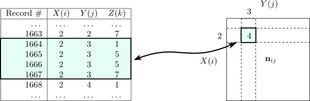
![]() . The contingency table has a direct
relationship to the list of observations; Figure 2.2 shows an
example where a list of observations of three variables is used to form a
two-variable contingency table.
. The contingency table has a direct
relationship to the list of observations; Figure 2.2 shows an
example where a list of observations of three variables is used to form a
two-variable contingency table.
|
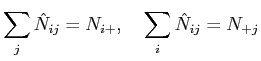
Any contingency table can be collapsed to a lower-dimensional table
by summing along one or more dimensions; a collapsed table is called a
marginal table or margin. The notation
![]() is used for
the margin where the second and third variables are collapsed, leaving only
the breakdown of the sample into the
is used for
the margin where the second and third variables are collapsed, leaving only
the breakdown of the sample into the ![]() categories of variable
categories of variable ![]() .
The + symbols in the notation indicate that the margin is derived by summing
.
The + symbols in the notation indicate that the margin is derived by summing
![]() over all categories
over all categories ![]() and
and ![]() . The total size of the
tabulated sample is given by
. The total size of the
tabulated sample is given by ![]() , or more typically by
, or more typically by ![]() alone.
alone.
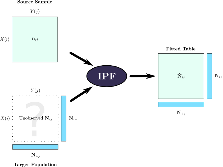
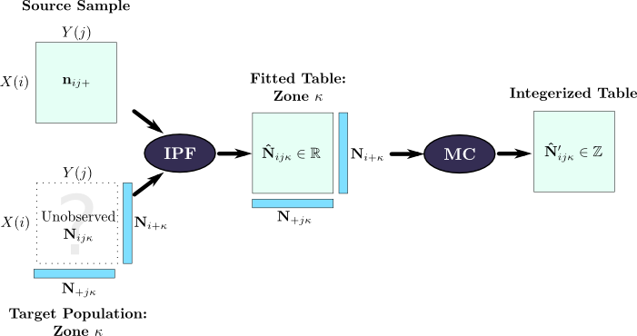
In this paper, multiple contingency tables are often considered simultaneously.
In a typical application of the Iterative Proportional Fitting (IPF)
procedure, a “source” population is sampled and cross-classified to
form a multiway table
![]() . A similarly structured
multiway table
. A similarly structured
multiway table
![]() is desired for some target population, but
less information is available about the target: typically, some marginal totals
is desired for some target population, but
less information is available about the target: typically, some marginal totals
![]() and
and
![]() are known. (Depending upon the
application, the target and source populations may be distinct or identical; in
a common example, the populations are identical but the source sample is small
(1-5%) while
the target margins may be a complete 100% sample of the population.) The
complete multiway table
are known. (Depending upon the
application, the target and source populations may be distinct or identical; in
a common example, the populations are identical but the source sample is small
(1-5%) while
the target margins may be a complete 100% sample of the population.) The
complete multiway table
![]() of the target population is
never known, but the IPF procedure is used to find an estimate
of the target population is
never known, but the IPF procedure is used to find an estimate
![]() . This is achieved through repeated modifications of the
table
. This is achieved through repeated modifications of the
table ![]() . The entire process and associated notation are shown in
Figure 2.3 and Table 2.1.
. The entire process and associated notation are shown in
Figure 2.3 and Table 2.1.
|
Note that the source table ![]() and target margins
and target margins ![]() are usually
integer counts, but the estimated target table
are usually
integer counts, but the estimated target table
![]() produced by
Iterative Proportional Fitting is real-valued.
produced by
Iterative Proportional Fitting is real-valued.
The Iterative Proportional Fitting (IPF) algorithm is generally attributed to Deming & Stephan [16]. (According to [14], it was preceded by a 1937 German publication applying the method to the telephone industry.) The method goes by many names, depending on the field and the context. Statisticians apply it to contingency tables and use the terms table standardization or raking. Transportation researchers use it for trip distribution and gravity models, and sometimes reference early papers in that field by Fratar or Furness [15,23]. Economists apply it to Input-Output models and call the method RAS [32].
|
Input: Source table
Output: Fitted table
![\begin{algorithm}
% latex2html id marker 693
[tb]\KwIn{Source table $\mathbf{n...
...ing procedure using a two-way table and one-way target margins.}
\end{algorithm}](img55.png)
|
The IPF algorithm is a method for adjusting a source
contingency table to match known marginal totals for some target population.
Figure 2.4 shows a simple application of IPF in two
dimensions. The table
![]() computed in
iteration
computed in
iteration ![]() fits the row totals exactly, with some error
in the column totals. In iteration
fits the row totals exactly, with some error
in the column totals. In iteration ![]() , an exact fit to the column
margins is achieved, but with some loss of fit to the row totals.
Successive iteration yields a fit to both target margins within some
tolerance
, an exact fit to the column
margins is achieved, but with some loss of fit to the row totals.
Successive iteration yields a fit to both target margins within some
tolerance ![]() . The procedure extends in a straightforward manner to
higher dimensions, and also with higher-dimensional margins.
. The procedure extends in a straightforward manner to
higher dimensions, and also with higher-dimensional margins.
Deming and Stephan [16] initially proposed the method to
account for variations in sampling accuracy. They imagined that the source
table and target marginals were measured on the same population, and that
the marginal totals were known exactly, but the source table had been
measured through a sampling process with some inaccuracy. The IPF method
would then adjust the sample-derived cells to match the more accurate marginal
totals. They framed this as a fairly general problem
with a ![]() -way contingency table, and considered both one-way margins
and higher-order margins (up to
-way contingency table, and considered both one-way margins
and higher-order margins (up to ![]() ways). They did not consider
the effect of zero values in either the initial cell values or the margins.
ways). They did not consider
the effect of zero values in either the initial cell values or the margins.
Deming and Stephan claimed that the IPF algorithm produces a unique solution that meets two criteria. It exactly satisfies the marginal constraints
Ireland and Kullback included a proof of convergence. It omitted one step, and was corrected by Csiszár in a 1975 paper [13]. Csiszár's treatment was somewhat more general than previous papers. In particular, he adopted a convention for the treatment of zero values in the initial cells:
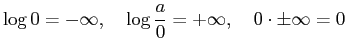 |
(7) |
The IPF method is one of several ways of satisfying the marginal
constraints (2.1) while minimizing entropy relative to
the source table. Alternative algorithms exist for solving this system of
equations, including Newton's method. Newton's method offers the advantage
of a faster (quadratic) convergence rate, and is also able to estimate
the parameters and
variance-covariance matrix associated with the system (to be discussed in
the following section). However, Newton's method is considerably less
efficient in computational storage and is impractical for the
large systems of equations that occur in high-dimensional problems.
Using the asymptotic Landau
![]() notation conventional in
computer science [11], the IPF method requires
notation conventional in
computer science [11], the IPF method requires
![]() memory to fit a
contingency table with
memory to fit a
contingency table with ![]() cells, while Newton's method requires
cells, while Newton's method requires
![]() storage [1, chapter 8], [20].
storage [1, chapter 8], [20].
Additionally, the minimum discrimination information of equation (2.6) is not the only possible optimization criterion for comparing the fitted table to the source table. Little & Wu [33] looked at a special case where the source sample and the target margins are drawn from different populations. In their analysis, they compared the performance of four different criteria: minimum discrimination information, minimum least squares, maximum log likelihood and minimum chi-squared. For certain problems, other optimization criteria may offer some advantages over minimum discrimination information.
In summary, the Iterative Proportional Fitting method is a data fusion technique for combining the information from a source multiway contingency table and lower-dimensional marginal tables for a target population. It provides an exact fit to the marginal tables, while minimizing discrimination information relative to the source table.
Following the basic understanding of the IPF method in the late 1960s and
early 1970s, the method received further attention in the statistical and
information theory community. As discussed earlier, Csiszár's 1975
paper [13] was in part a correction and generalization of Ireland
& Kullback's work. However, it also introduced a different conception of
the underlying problem. Csiszár did not represent the multiway
probability distribution as a ![]() -way contingency table with
-way contingency table with ![]() cells.
Instead, he conceived of
cells.
Instead, he conceived of ![]() -space, a much larger
-space, a much larger ![]() -dimensional space
containing all possible probability distributions for the
-dimensional space
containing all possible probability distributions for the ![]() cells in the
contingency table. He exploited the geometric properties of this space to
prove convergence of the algorithm.
cells in the
contingency table. He exploited the geometric properties of this space to
prove convergence of the algorithm.
The mechanics of his proof and construction of ![]() -space would be a
theoretical footnote, except that further extensions and generalizations of
the IPF method have been made using the
-space would be a
theoretical footnote, except that further extensions and generalizations of
the IPF method have been made using the ![]() -space notation and
conceptualization. In
-space notation and
conceptualization. In ![]() -space, the marginal constraints form closed linear
sets. The IPF algorithm is described as a series of
-space, the marginal constraints form closed linear
sets. The IPF algorithm is described as a series of ![]() -projections onto
these linear constraints.
-projections onto
these linear constraints.
From a cursory reading of a 1985 paper by Dykstra [17], it appears
that he generalized Csiszár's theory and proved convergence of the IPF
method for a broader class of constraints: namely any closed, convex set
in ![]() -space. Dykstra used a complicated example where the cells are not
constrained to equal some marginal constraint, but the tables' marginal
total vectors were required to satisfy an ordering constraint—for
example, requiring that
-space. Dykstra used a complicated example where the cells are not
constrained to equal some marginal constraint, but the tables' marginal
total vectors were required to satisfy an ordering constraint—for
example, requiring that
![]() . Dykstra's
iterative procedure was broadly the same as the IPF procedure: an iterative
projection onto the individual convex constraints. In other words, small
extensions to the IPF method can allow it to satisfy a broader class of
constraints beyond simple equality.
. Dykstra's
iterative procedure was broadly the same as the IPF procedure: an iterative
projection onto the individual convex constraints. In other words, small
extensions to the IPF method can allow it to satisfy a broader class of
constraints beyond simple equality.
Further generalizations of the IPF method are discussed by Fienberg & Meyer [20].
Log-linear models provide a means of statistically analyzing patterns of association in a single contingency table. They are commonly used to test for relationships between different variables when data is available in the form of a simple, low-dimensional contingency table. The method itself derives from work on categorical data and contingency tables in the 1960s that culminated in a series of papers by Goodman in the early 1970s [19]. The theory behind log-linear models is well-established and is described in detail elsewhere [54,1,37]. In this section, a few examples are used to provide some simple intuition for their application. The notation used here follows [54], but is fairly similar to most sources.
Consider a single two-dimensional contingency table
![]() containing
observations of variables
containing
observations of variables ![]() and
and ![]() . The general form
of a log-linear model for such a table is
. The general form
of a log-linear model for such a table is
| (8) |
| (9) |
| (10) |
| for all |
||
| for some |
(11) |
As more variables are added, higher-order association patterns such as
![]() can be included, and the number of possible models grows.
In practise, only hierarchical models are used, where an association
term
can be included, and the number of possible models grows.
In practise, only hierarchical models are used, where an association
term
![]() is only included when lower-order terms
is only included when lower-order terms ![]() and
and ![]() are also included.
Hierarchical models are usually summarized using only their highest-order
terms. For example, the model
are also included.
Hierarchical models are usually summarized using only their highest-order
terms. For example, the model
![]() implicitly includes
implicitly includes ![]() and
and ![]() terms.
For a given set of variables, the model that includes all possible
association terms is called the saturated model.
terms.
For a given set of variables, the model that includes all possible
association terms is called the saturated model.
To ensure uniqueness, constraints are usually applied to the parameters of a log-linear model. Two different conventions are common, and tools for estimating log-linear models may use either convention. The ANOVA-type coding or effect coding using the following constraints for a two-way table [37]:
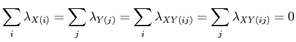 |
(12) |
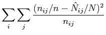
After estimating the parameters of a log-linear model based on observed
counts ![]() , the estimated counts
, the estimated counts
![]() are obtained. The model
fits can be tested on these estimates using either the Pearson statistic
are obtained. The model
fits can be tested on these estimates using either the Pearson statistic
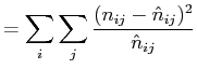 |
(13) |
 |
(14) |
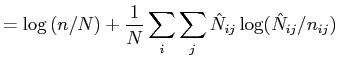
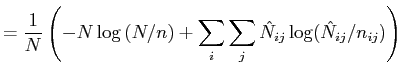
Finally, the ![]() statistic for the null model (
statistic for the null model (
![]() ) is
related to the entropy of a probability distribution. The formula for
entropy is
) is
related to the entropy of a probability distribution. The formula for
entropy is
 |
(15) | |
|
and can be translated to a table of counts as
| ||
 |
(16) | |
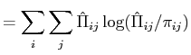
The Iterative Proportional Fitting procedure has long been associated with
log-linear analysis. Given a log-linear model and a contingency table
![]() , it is often useful to know what the fitted table of
frequencies
, it is often useful to know what the fitted table of
frequencies
![]() would be under the model. (For intuitive
purposes, this is the equivalent of finding the shape of the fitted line
under the model of linear regression.)
would be under the model. (For intuitive
purposes, this is the equivalent of finding the shape of the fitted line
under the model of linear regression.)
In this problem, a log-linear model is called direct if the fitted
table can be expressed as closed formulae, or indirect if
the fitting can only be achieved using an iterative algorithm. For indirect
models such as
![]() , IPF has long been employed as an efficient way to
fit a table to the data. To achieve this, the source table
, IPF has long been employed as an efficient way to
fit a table to the data. To achieve this, the source table
![]() is chosen to have no pattern of association whatsoever; typically, this is
done by setting
is chosen to have no pattern of association whatsoever; typically, this is
done by setting ![]() . The target margins used by the IPF
procedure are the “minimal sufficient statistics” of the log-linear
model; for example, to fit the model
. The target margins used by the IPF
procedure are the “minimal sufficient statistics” of the log-linear
model; for example, to fit the model
![]() , the marginal tables
, the marginal tables
![]() and
and
![]() would be applied. The resulting table
found by IPF is known to give the maximum likelihood fit.
would be applied. The resulting table
found by IPF is known to give the maximum likelihood fit.
Each step of the IPF procedure adjusts all cells contributing to a given marginal cell equally. As a result, it does not introduce any new patterns of association that were not present in the source table; and the source table was chosen to include no association whatsoever. The resulting table shows only the modelled patterns of association [54, §5.2].
The IPF procedure is hence an important tool for log-linear modelling.
Additionally, log-linear models provide some useful insight into the
behaviour of the IPF procedure. Stephan
showed that the relationship between the fitted table
![]() and the source table
and the source table
![]() could be expressed as
could be expressed as
This view of the IPF procedure is mostly useful for interpreting its
behaviour. IPF modifies the source table
![]() to create a fitted
table
to create a fitted
table
![]() ; that change, represented by the left hand side
of equation (2.18), can be expressed using a small number of parameters
(the various
; that change, represented by the left hand side
of equation (2.18), can be expressed using a small number of parameters
(the various ![]() terms). The number of parameters necessary is directly
proportional to the size of the marginal tables used in the fitting
procedure; in this case,
terms). The number of parameters necessary is directly
proportional to the size of the marginal tables used in the fitting
procedure; in this case,
![]() .
This insight is not unique to log-linear models, but it is perhaps easier
to understand than the Lagrangian analysis used in early IPF papers.
.
This insight is not unique to log-linear models, but it is perhaps easier
to understand than the Lagrangian analysis used in early IPF papers.
The only shortcoming of the preceding discussion of IPF and log-linear models concerns zeros in the source table or target margins. While Csiszár's treatment of zeros allows the IPF procedure to handle zeros elegantly, it remains difficult to determine the correct number of parameters used by IPF when either the source or target tables contain zeros.
The zeros can take the form of either structural or sampling zeros. Structural zeros occur when particular combinations of categories are impossible. For example, if a sample of women is cross-classified by age and by number of children, the cell corresponding to “age 0-10” and “1 child” would be a structural zero (as would all higher number of children for this age group). A sampling zero occurs when there is no a priori reason that a particular combination of categories would not occur, but the sample was small enough that no observations were recorded for a particular cell.
Wickens provides a detailed description of the consequences of zero cells for log-linear modelling [54, §5.6]. For high dimensional tables, the number of parameters in a particular model becomes difficult to compute, and this in turn makes it difficult to determine how many degrees of freedom are present. As he notes, however, “The degrees of freedom are off only for global tests of goodness of fit and for tests of the highest-order interactions.” Clogg and Eliason suggested that goodness-of-fit tests are futile when the data becomes truly sparse:
But there is a sense in which goodness-of-fit is the wrong question to ask when sparse data is analyzed. It is simply unreasonable to expect to be able to test a model where there are many degrees of freedom relative to the sample size. [10]
For a small number of zeros, then, it seems that some log-linear analysis may be possible. A sparse table with a large number of zeros, by contrast, is unlikely to be tested for goodness-of-fit.
Microsimulation and agent-based methods of systems modelling forecast the future state of some aggregate system by simulating the behaviour of a number of disaggregate agents over time [9].
In many agent-based models where the agent is a person, family or household the primary source of data for population synthesis is a national census. In many countries, the census provides two types of data about these agents. Large-sample detailed tables of one or two variables across many small geographic areas are the traditional form of census delivery, and are known as Summary Files in the U.S., Profile Tables or Basic Summary Tabulations (BSTs) in Canada, and Small Area Statistics in the U.K. In addition, a small sample of individual census records is now commonly available in most countries. These samples consist of a list of individuals (or families or households) drawn from some large geographic area, and are called Public-Use Microdata Samples (PUMS) in the U.S. and Canada, or a Sample of Anonymized Records in the U.K. The geographic area associated with a PUMS is the Public-Use Microdata Area (PUMA) in the U.S., and the Census Metropolitan Area (CMA) in Canada. The population synthesis procedure can use either or both of these data sources, and must produce a list of agents and their attributes, preferably at a relatively fine level of geographic detail.
In this document, the terms Summary Tables, PUMS and PUMA will be used. For small areas inside a PUMA, the Census Tract (CT) will often be used (or more generically a “zone”), but any fine geographic unit that subdivides the PUMA could be used. Further details about the data and definitions are presented in Chapter 3.
In most population synthesis procedures, geography receives special attention. This is not because geography is inherently different than any other agent attribute: like the other attributes, location is treated as a categorical variable, with a fine categorization system (small zones like census tracts) that can be collapsed to a coarse set of categories (larger zones, like the Canadian Census Subdivisions), or even collapsed completely (to the full PUMA) to remove any geographic variation. There are two reasons why geography receives special attention: first, because census data is structured to treat geography specially. One data set (the PUMS) provides data on the association between almost all attributes except geography; the other (Summary Tables) includes geography in every table, and gives its association with one or two other variables. Secondly, geography is one of the most important variables for analysis and often has a large number of categories; while an attribute like age can often be reduced to 15-20 categories, reducing geography to such a small number of categories would lose a substantial amount of variation that is not captured in other attributes. For transportation analysis, a fine geographic zone system is essential for obtaining a reasonable representation of travel distances, access to transit systems, and accurate travel demand. As a result, geography is usually broken up into hundreds of zones, sometimes more than a thousand.
 |
The Iterative Proportional Fitting method is the most popular means for
synthesizing a population. The simplest approach is to consider each
small geographic zone independently. Suppose that the geographic zones are
census tracts contained in some PUMA. Further, suppose that each agent needs
two attributes ![]() and
and ![]() , in addition to a zone identifier
, in addition to a zone identifier ![]() .
An overview of the process is shown in Figure 2.5.
.
An overview of the process is shown in Figure 2.5.
The synthesis is conducted one zone at a time, and the symbol ![]() denotes the zone of interest. In the simplest approach,
the variables
denotes the zone of interest. In the simplest approach,
the variables ![]() and
and ![]() are assumed to have no association pattern (i.e.,
they are assumed to vary independently), and hence the initial table
are assumed to have no association pattern (i.e.,
they are assumed to vary independently), and hence the initial table
![]() is set to a constant value of one.
The summary tables provide the known information about zone
is set to a constant value of one.
The summary tables provide the known information about zone ![]() :
the number of individuals in each category of variable
:
the number of individuals in each category of variable ![]() can be tabulated
to form
can be tabulated
to form
![]() , and likewise with variable
, and likewise with variable ![]() to give
to give
![]() . These are used as the target margins for the IPF
procedure, giving a population estimate for zone
. These are used as the target margins for the IPF
procedure, giving a population estimate for zone ![]() .
.
However, the variables ![]() and
and ![]() are unlikely to be independent. The PUMS
provides information about the association between the variables, but
for a different population: a small sample in the geographically larger
PUMA. As discussed by Beckman, Baggerly & McKay
[4], under the
assumption that the association between
are unlikely to be independent. The PUMS
provides information about the association between the variables, but
for a different population: a small sample in the geographically larger
PUMA. As discussed by Beckman, Baggerly & McKay
[4], under the
assumption that the association between ![]() and
and ![]() in zone
in zone ![]() is the
same as the association in the PUMA, the initial table
is the
same as the association in the PUMA, the initial table
![]() can be set to a cross-classification of the PUMS over variables
can be set to a cross-classification of the PUMS over variables ![]() and
and ![]() . IPF is then applied, yielding a different result.
. IPF is then applied, yielding a different result.
The IPF process produces a multiway contingency table for zone ![]() , where each
cell contains a real-valued “count”
, where each
cell contains a real-valued “count”
![]() of the number of
agents with a particular set of attributes
of the number of
agents with a particular set of attributes ![]() and
and ![]() . However, to
define a discrete set of agents integer counts are required. Rounding the
counts is not a satisfactory “integerization” procedure for three reasons:
the rounded table may not be the best solution in terms of discrimination
information; the rounded table may not offer as good a fit to margins as other
integerization procedures; and rounding may bias the estimates.
. However, to
define a discrete set of agents integer counts are required. Rounding the
counts is not a satisfactory “integerization” procedure for three reasons:
the rounded table may not be the best solution in terms of discrimination
information; the rounded table may not offer as good a fit to margins as other
integerization procedures; and rounding may bias the estimates.
Beckman et al. handled this problem by treating the fitted table as a
joint probability mass function (PMF), and then used ![]() Monte Carlo
draws [24] from this PMF to select
Monte Carlo
draws [24] from this PMF to select ![]() individual cells. These
draws can be
tabulated to give an integerized approximation
individual cells. These
draws can be
tabulated to give an integerized approximation
![]() of
of
![]() . This is an effective way
to avoid biasing problems, but at the expense of introducing a nondeterministic step into the synthesis.
. This is an effective way
to avoid biasing problems, but at the expense of introducing a nondeterministic step into the synthesis.
Finally, given an integer table of counts, individual agents can be
synthesized using lookups from the original PUMS list. (See
Figure 2.2 for an illustration of the link between the list and
tabular representations.) Beckman et al. observed an important aspect of
this process: if ![]() is zero (i.e., no records in the PUMS for a
particular combination of variables), then the fitted count
is zero (i.e., no records in the PUMS for a
particular combination of variables), then the fitted count
![]() will be zero, and this carries through to the
integerized count
will be zero, and this carries through to the
integerized count
![]() . Consequently, any cell in
. Consequently, any cell in
![]() that has a non-zero count is guaranteed to have
corresponding individual(s) in the PUMS.
that has a non-zero count is guaranteed to have
corresponding individual(s) in the PUMS.
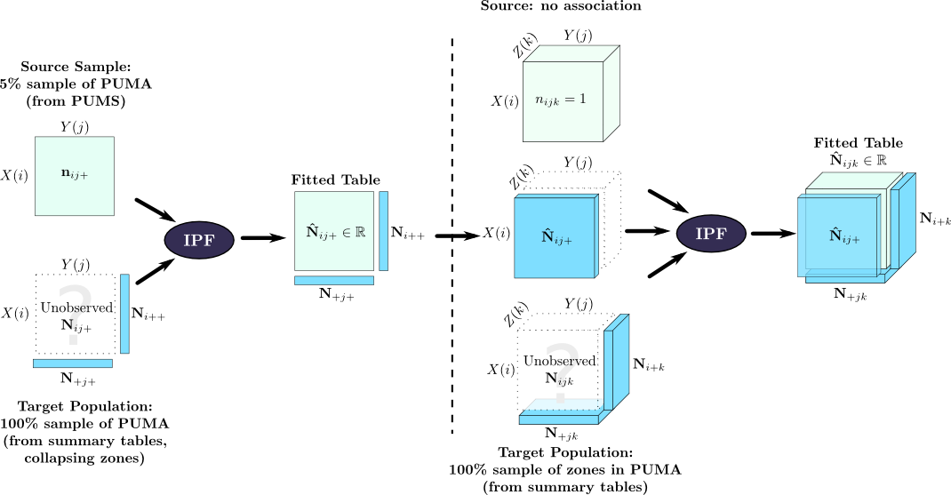
Beckman, Baggerly & McKay [4] discussed the simple zone-by-zone technique and also extended it to define a multizone estimation procedure; their approach has been widely cited [5,21,2] and is described in great detail by [27]. They described a method for using IPF with a PUMS to synthesize a set of households. Their approach addresses a weakness of the zone-by-zone method: the PUMS describes the association pattern for a large geographic area, and the pattern within small zones inside that area may not be identical. Consequently, Beckman et al. made no assumptions about the association pattern of the individual zones, but instead required the sum over all zones to match the PUMS association pattern. This approach is illustrated graphically in Figure 2.6; their paper includes a more detailed numerical example. (The Monte Carlo integerization step is omitted for clarity.)
|
This multizone approach offers an important advantage over the zone-by-zone approach. The zone-by-zone approach uses the PUMS association pattern for the initial table, but it is overruled by the marginal constraints, and its influence on the final result is limited. By applying the PUMS association pattern as a marginal constraint on the IPF procedure, the multizone method guarantees that the known association pattern in the PUMS is satisfied exactly.
Many projects have applied Beckman et al.'s methods. Most microsimulation projects seem to use a zone-by-zone fitting procedure with a PUMS, followed by Monte Carlo draws as described by Beckman. Few seem to have adopted Beckman's multizone fitting procedure, however. This may be due to storage limitations: synthesizing all zones simultaneously using Beckman's multizone method requires substantially more computer memory, and would consequently limit the number of other attributes that could be synthesized.
In terms of different agent types, Beckman et al. considered households,
families and individuals in a single unit. They segmented households into
single-family, non-family and group quarters. They then synthesized family
households, including a few individual characteristics (age of one
family member) and “presence-of-children” variables. They did not
synthesize person agents explicitly, did not associate families with
dwellings, and did not synthesize the connection between families in
multifamily households. Later work on their model (TRANSIMS) did synthesize
persons from the households [27].
Their largest table was for family households with ![]() variables and
variables and
![]() cells before including geography, of which 609 cells were nonzero.
Their sample was a 5% sample of a population of roughly 100,000 individuals.
cells before including geography, of which 609 cells were nonzero.
Their sample was a 5% sample of a population of roughly 100,000 individuals.
Guo & Bhat [26] applied Beckman's procedure to a population of households in the Dallas-Fort Worth area in Texas. (It is not clear whether they used zone-by-zone synthesis or applied Beckman's multizone approach.) They modified Beckman's integerization procedure by making Monte Carlo draws without replacement, with some flexibility built into the replacement procedure in the form of a user-defined threshold. Further, they proposed a procedure for simultaneously synthesizing households and individuals. In their procedure, the household synthesis includes some information about the individuals within the household: the number of persons and the family structure. A series of individuals are synthesized to attach to the household, using the limited known information from the synthesized household. If any of the synthetic individuals are “improbable” given the number of demographically similar individuals already synthesized, then the entire household is rejected and resynthesized.
The linkage between households and individuals in this method remains weak, and the procedure is fairly ad hoc. Guo & Bhat showed that the method did improve fit in the individual table fits during a single trial, but the results were not adequate for any conclusive claims.
Huang & Williamson [28] implemented an IPF-based method for comparison against the Combinatorial Optimization method. They used a novel zone-by-zone synthesis procedure. In their approach, large zones (“wards”) within a PUMA were first synthesized one-at-a-time, under the assumption that each ward has the same association pattern as the larger PUMA. The ward results were then used as the initial table for the synthesis of finer zones (enumeration districts) within each ward. This multilevel approach improves on the conventional zone-by-zone method.
Huang & Williamson also used an incremental approach to attribute synthesis which they call “synthetic reconstruction” where after an initial fitting to produce four attributes, additional attributes are added one-at-a-time. The motivation for this approach is apparently to avoid large sparse tables, and includes collapsing variables to coarser categorization schemes to reduce storage requirements and sparsity. However, their method is complex and requires substantial judgment to construct a viable sequencing of new attributes, by leveraging a series of conditional probabilities. Furthermore, the connection to the PUMS agents is lost: the resulting population is truly synthetic, with some new agents created that do not exist in the initial PUMS. Since only a subset of the attributes are considered at a time, it is possible that some attributes in the synthetic agents may be contradictory. Nevertheless, the analysis is interesting, and reveals the effort sometimes expended when trying to apply IPF rigorously to obtain a population with a large number of attributes.
Finally, Huang & Williamson proposed a modification to the Monte Carlo procedure, by separating the integer and fractional components of each cell in the multiway table. The integer part is used directly to synthesize discrete agents, and the table of remaining fractional counts is then used for Monte Carlo synthesis of the final agents.
The primary alternative to the Iterative Proportional Fitting algorithm is the reweighting approach advocated by Williamson. In a 1998 paper [57], Williamson et al. proposed a zone-by-zone method with a different parameterization of the problem: instead of using a contingency table of real-valued counts, they chose a list representation with an integer weight for each row in the PUMS. (As illustrated in Figure 2.2, there is a direct link between tabular and list-based representations.)
For each small zone ![]() within a PUMA, the zone population
is much smaller than the observations in the PUMS; that is,
within a PUMA, the zone population
is much smaller than the observations in the PUMS; that is,
![]() . This made it possible for Williamson et al. to
to choose a subset of the PUMS to represent the population of the zone,
with no duplication of PUMS agents in the zone. In other words, the weight
attached to each agent is either zero or one (for a single zone).
. This made it possible for Williamson et al. to
to choose a subset of the PUMS to represent the population of the zone,
with no duplication of PUMS agents in the zone. In other words, the weight
attached to each agent is either zero or one (for a single zone).
To estimate the weights, they used various optimization procedures to find the set of 0/1 weights yielding the best fit to the Summary Tables for a single zone. They considered several different measures of fit, and compared different optimization procedures including hill-climbing, simulated annealing and genetic algorithms. By solving directly for integer weights, Williamson obtained a better fit to the Summary Tables than Beckman et al., whose Monte Carlo integerization step harmed the fit.
Williamson et al. [57] proposed three primary reasons motivating their approach:
The last two claims are somewhat weak. It is true that many IPF procedure require coarse categorization during fitting, in order to conserve limited memory. However, after completion, Beckman's approach does produce a list of PUMS records (and can be linked to other data sources easily). Even if a coarse categorization was used during fitting, it is still possible to use the fine categorization in the PUMS after synthesis. Nevertheless, IPF does require a carefully constructed category system to make fitting possible, and this can be time-consuming to design and implement.
The reweighting approach has three primary weaknesses. First, the attribute
association observed in the PUMS (
![]() ) is not preserved by the
algorithm. The IPF method has an explicit formula defining the relationship
between the fitted table
) is not preserved by the
algorithm. The IPF method has an explicit formula defining the relationship
between the fitted table
![]() and the PUMS table
and the PUMS table
![]() in equation (2.18). Beckman et al.'s
multizone approach also treats the PUMS association pattern for the entire
PUMA as a constraint, and ensures that the full population matches that
association pattern. The reweighting method does operate on the PUMS, and
an initial random choice of weights will match the association pattern of
the PUMS. However, the reweighting procedure does not make any effort to
preserve that association pattern.
While the reweighting method has been evaluated in many ways
[52,28,56,38], it does not appear that the fit
to the PUMS at the PUMA level has been tested.
in equation (2.18). Beckman et al.'s
multizone approach also treats the PUMS association pattern for the entire
PUMA as a constraint, and ensures that the full population matches that
association pattern. The reweighting method does operate on the PUMS, and
an initial random choice of weights will match the association pattern of
the PUMS. However, the reweighting procedure does not make any effort to
preserve that association pattern.
While the reweighting method has been evaluated in many ways
[52,28,56,38], it does not appear that the fit
to the PUMS at the PUMA level has been tested.
Secondly, the reweighting method is very computationally expensive. When
solving for a single zone ![]() , there are
, there are ![]() 0/1 weights, one for each
PUMS entry. However, this gives rise to
0/1 weights, one for each
PUMS entry. However, this gives rise to
![]() possible
combinations; “incredibly large,” in the authors' words
[57]. Of course, the optimization procedures are intelligent
enough to explore this space selectively and avoid an exhaustive search;
nevertheless, the authors reported a runtime of 33 hours using an 800MHz
processor [28]. Since the number of permutations grows
factorially with the number of individuals in the zone, it is not
surprising that the authors chose to work with the smallest zones possible
(1440 zones containing an average of 150 households each); it is possible
that larger zones would not be feasible.
possible
combinations; “incredibly large,” in the authors' words
[57]. Of course, the optimization procedures are intelligent
enough to explore this space selectively and avoid an exhaustive search;
nevertheless, the authors reported a runtime of 33 hours using an 800MHz
processor [28]. Since the number of permutations grows
factorially with the number of individuals in the zone, it is not
surprising that the authors chose to work with the smallest zones possible
(1440 zones containing an average of 150 households each); it is possible
that larger zones would not be feasible.
Finally, the reweighting method uses
![]() weights to represent a
weights to represent a
![]() -zone area. This parameter space is quite large; larger, in fact, than
the population itself. It is not surprising that good fits can be achieved
with a large number of parameters, but the method is not particularly
parsimonious and may overfit the Summary Tables. It is likely that
a simpler model with fewer parameters could achieve as good a fit, and
would generalize better from the 2% PUMS sample to the full
population.
-zone area. This parameter space is quite large; larger, in fact, than
the population itself. It is not surprising that good fits can be achieved
with a large number of parameters, but the method is not particularly
parsimonious and may overfit the Summary Tables. It is likely that
a simpler model with fewer parameters could achieve as good a fit, and
would generalize better from the 2% PUMS sample to the full
population.