Next: 6. Results Up: thesis Previous: 4. The Disparity Map Contents
The parameterisation of the cloth surface follows several stages, similar in principle to stages in many computer vision systems. First, features are detected in the intensity image. Each feature is then matched with features in a flat reference image of the cloth. The global structure of the parameterisation is analysed, and invalid features are rejected. Finally, parameter values are interpolated for every pixel in the input image.
For feature detection, we use Lowe's Scale-Invariant Feature Transform (SIFT) [76,77]. Features detected using SIFT are largely invariant to changes in scale, illumination, and local affine distortions. Each feature has an associated scale, orientation and position, measured to subpixel accuracy. Features are found at edges using the scale-space image gradient. Each feature has a high-dimensional "feature vector,'' which consists of a coarse multiscale sampling of the local image gradient. The Euclidean distance between two feature vectors provides an estimate of the features' similarity. Lowe used SIFT features for the object recognition task, and considered only rigid objects with a very small number of degrees of freedom. See Brown and Lowe's 2002 paper [21] for an example of object recognition. An upcoming paper by the same authors [22] uses SIFT for image registration in panorama stitching, a very different problem. We make heavy use of SIFT features, but we must adapt the matching to the parameterisation of cloth, a deformable surface with a very high number of degrees of freedom.
We detect features in two different images. A scan of the
flattened cloth is used
to obtain the reference image, a flat and undistorted view of
the cloth. We use the 2D image coordinates of points in the reference image
directly as (u,v) parameters for the features. This 2D parametric reference space is denoted
![]() .
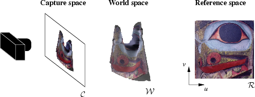
The second image is the input intensity image, called the captured
image here. We refer to this 2D image space as the capture space, and denote it
.
The second image is the input intensity image, called the captured
image here. We refer to this 2D image space as the capture space, and denote it
![]() .
.
We also work in world space
![]() , the
three-dimensional space imaged by the stereo system. Capture
space is a perspective projection of world space,
and the disparity map provides a discretised mapping from
capture space to world space. We map disparity values at discrete
locations back to world space and use linear interpolation
to obtain a continuous mapping. Finally, we also
work in the feature space
, the
three-dimensional space imaged by the stereo system. Capture
space is a perspective projection of world space,
and the disparity map provides a discretised mapping from
capture space to world space. We map disparity values at discrete
locations back to world space and use linear interpolation
to obtain a continuous mapping. Finally, we also
work in the feature space
![]() . This is a
128-dimensional space containing the SIFT feature vectors for both the
reference and the captured features.
. This is a
128-dimensional space containing the SIFT feature vectors for both the
reference and the captured features.
 |
After applying SIFT to the reference and captured images, we obtain two sets of features,
If we can establish a one-to-one mapping between reference features and
captured features, then we know both the world space position and
the reference space position of every captured feature, allowing
parameterisation. In the matching stage of the algorithm described in
Section 5.2, we construct this one-to-one mapping, which we label
![]() . It should be noted that a
one-to-one mapping is only feasible if the pattern in the reference image
has no repetitions.
. It should be noted that a
one-to-one mapping is only feasible if the pattern in the reference image
has no repetitions.
Cloth strongly resists stretching, but permits substantial bending; folds and wrinkles are a distinctive characteristic of cloth. This behaviour means that sections of the cloth are often seen at oblique angles, leading to large affine distortions of features in certain regions of the cloth. Unfortunately, SIFT features are not invariant to large affine distortions.
To compensate for this, we use an expanded set of reference
features. We generate a new reference image by using a 2×2
transformation matrix T to scale the reference image by
half horizontally. We repeat three more times, scaling vertically and
along axes at ![]() 45°, as shown in Figure 5.3. This
simulates different oblique views of the reference image. For each of
these scaled oblique views, we collect a set of SIFT
features. Finally, these new SIFT features are merged into the
reference feature set. When performing this merge, we must adjust feature
positions, scales and orientations by using
45°, as shown in Figure 5.3. This
simulates different oblique views of the reference image. For each of
these scaled oblique views, we collect a set of SIFT
features. Finally, these new SIFT features are merged into the
reference feature set. When performing this merge, we must adjust feature
positions, scales and orientations by using
![]() .
This approach is compatible with the recommendations made by Lowe [77]
for correcting SIFT's sensitivity to affine change.
.
This approach is compatible with the recommendations made by Lowe [77]
for correcting SIFT's sensitivity to affine change.
![\includegraphics[width=.7\linewidth]{totem1}](totem1.png) |
The Euclidean distance in
![]() given by
given by
![]() is the simplest metric for finding a
match between a reference feature
is the simplest metric for finding a
match between a reference feature
![]() and a given
captured feature
and a given
captured feature
![]() . Unfortunately, in our tests with
cloth this metric is not sufficient for good matching, and tends to
produce a sizable number of incorrect matches.
. Unfortunately, in our tests with
cloth this metric is not sufficient for good matching, and tends to
produce a sizable number of incorrect matches.
We would like to enforce an additional constraint while performing feature matching. The spatial relationship between features can help to eliminate bad matches: any pair of features that are close in reference space must have matches which are close in capture space. The converse is not always true, since two nearby captured features may lie on opposite sides of a fold. If we could enforce this capture/reference distance constraint during the matching process, we could obtain better results.
We can extend this notion by thinking about distances between features
in world space. Suppose that we have complete knowledge of the cloth surface
in world space (including occluded areas), and can calculate the
geodesic distance in
![]() between two captured features
between two captured features
![]() :
:
Now, consider two reference features
![]() , which are
hypothetical matches for cs and cn. We know the distance in
, which are
hypothetical matches for cs and cn. We know the distance in
![]() between rs and rn, but we do not know the distance between them in
between rs and rn, but we do not know the distance between them in
![]() . By performing a simple calibration step, we can establish a
scalar multiple relating distances in these two spaces. We will multiply by
αr to map a distance from
. By performing a simple calibration step, we can establish a
scalar multiple relating distances in these two spaces. We will multiply by
αr to map a distance from
![]() to
to
![]() , and
multiply by αr-1 for the opposite mapping.
, and
multiply by αr-1 for the opposite mapping.
Using αr, the world space distance between the reference features can be calculated.
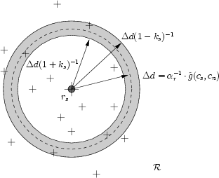
We refer to the lower bound on
![]() as the compression constraint,
and the upper bound is called the stretch constraint. If
as the compression constraint,
and the upper bound is called the stretch constraint. If
![]() , then this choice of match implies that the
captured cloth is very stretched; similarly, if the compression constraint is
violated, then this choice of match implies that the captured cloth is very
compressed. Provided that a reasonable choice is made for ks, we can
safely reject matches that violate the stretch constraint or the
compression constraint.
Figure 5.4 illustrates these constraints.
, then this choice of match implies that the
captured cloth is very stretched; similarly, if the compression constraint is
violated, then this choice of match implies that the captured cloth is very
compressed. Provided that a reasonable choice is made for ks, we can
safely reject matches that violate the stretch constraint or the
compression constraint.
Figure 5.4 illustrates these constraints.
 |
In our real-world setting, finding the geodesic distance between
captured features is more difficult. In situations where the entire
cloth surface between cs and cn is visible, we define a straight
line between cs and cn in
![]() , project this line onto
the surface in
, project this line onto
the surface in
![]() , and integrate along the line. This will
not find the geodesic distance, but will closely approximate it.
, and integrate along the line. This will
not find the geodesic distance, but will closely approximate it.
In some situations, sections of the cloth surface on the geodesic line
between cs and cn will be occluded. We can detect such situations using
the same line integration method as before, scanning for discontinuities in
depth along the line. When occlusion occurs, there is no way of estimating the
actual geodesic distance
![]() . However, we can still use
. However, we can still use
![]() , which in this case is likely to be an underestimate of
, which in this case is likely to be an underestimate of
![]() . The stretch constraint can be applied
to these features, but we cannot use the compression constraint, since the
amount of fabric hidden in the fold is unknown at this point.
. The stretch constraint can be applied
to these features, but we cannot use the compression constraint, since the
amount of fabric hidden in the fold is unknown at this point.
In contrast to the distance metric in feature space, the stretch and compression constraints are applied to pairs of matched features. To accommodate this, we adopt a seed-and-grow approach. First, a small number of seeds are selected, and these seeds are then matched using only the feature space distance metric. For each seed, we "grow'' outwards in capture space, finding nearby features and matching them. As we find features, we can use a nearby pre-matched feature to enforce the stretch constraint.
The seeding process is straightforward. We select a small subset of captured
features
![]() , and find matches for them in a
brute force manner. For each
, and find matches for them in a
brute force manner. For each
![]() , we compare against the
entire reference feature set Fr, and we use the feature-space
distance between c and
, we compare against the
entire reference feature set Fr, and we use the feature-space
distance between c and
![]() to define the quality of a match.
To improve the speed of the brute force matching, we use Beis & Lowe's
best bin first algorithm [9]; this is an approximate
search in a k-d tree. (It is approximate in that it always returns a
close match, but not always the best match possible.)
We then sort Fc' by the feature-space distance, and apply the
growth process on each seed in order, from best-matched to worst.
The growth process classifies captured features into three sets: matched,
rejected and unknown. If a seed fails to grow, the seed itself is classified as
rejected. After all seeds have been grown or rejected, we construct a
new Fc' from the remaining unknown captured features.
to define the quality of a match.
To improve the speed of the brute force matching, we use Beis & Lowe's
best bin first algorithm [9]; this is an approximate
search in a k-d tree. (It is approximate in that it always returns a
close match, but not always the best match possible.)
We then sort Fc' by the feature-space distance, and apply the
growth process on each seed in order, from best-matched to worst.
The growth process classifies captured features into three sets: matched,
rejected and unknown. If a seed fails to grow, the seed itself is classified as
rejected. After all seeds have been grown or rejected, we construct a
new Fc' from the remaining unknown captured features.
To help the process, we prefer captured features with a large SIFT
scale s(c) when selecting
![]() . In the first
iteration,
. In the first
iteration,
![]() consists of the largest features, followed
by a smaller group, and so on until a minimum scale is reached. Large
features are only found in relatively flat, undistorted, and
unoccluded regions of the cloth. In these regions, the growth process
will be able to proceed rapidly without encountering folds or
occlusions, rapidly reducing the number of unknown features. This
rapid growth reduces the number of features which must be considered
as seed candidates. The use of the seeding process should be reduced
as much as possible, since it cannot
make use of the stretch and compression constraints, and hence must
resort to relatively inefficient and unreliable brute force matching.
consists of the largest features, followed
by a smaller group, and so on until a minimum scale is reached. Large
features are only found in relatively flat, undistorted, and
unoccluded regions of the cloth. In these regions, the growth process
will be able to proceed rapidly without encountering folds or
occlusions, rapidly reducing the number of unknown features. This
rapid growth reduces the number of features which must be considered
as seed candidates. The use of the seeding process should be reduced
as much as possible, since it cannot
make use of the stretch and compression constraints, and hence must
resort to relatively inefficient and unreliable brute force matching.
The growth process is controlled with a priority queue. Each entry in the
priority queue is a matched source feature
![]() on the
edge of the growth region. The queue is sorted by capture space distance from
the seed, ensuring an outward growth from the seed. The queue is initialised
with the seed point alone. The source features are extracted from the queue
one at a time.
on the
edge of the growth region. The queue is sorted by capture space distance from
the seed, ensuring an outward growth from the seed. The queue is initialised
with the seed point alone. The source features are extracted from the queue
one at a time.
Let us consider one such source feature, consisting of cs and
![]() . To grow outwards, we iterate over all features
cn in the neighbourhood N(cs) of cs in capture space.
N(cs) is a circle of radius rc centred on cs.
For a given cn, the match candidates are the reference space
features which pass the stretch and compression constraints. These
candidate features lie in a ring around rs, as shown in
Figure 5.4.
. To grow outwards, we iterate over all features
cn in the neighbourhood N(cs) of cs in capture space.
N(cs) is a circle of radius rc centred on cs.
For a given cn, the match candidates are the reference space
features which pass the stretch and compression constraints. These
candidate features lie in a ring around rs, as shown in
Figure 5.4.
To select the best match among the match candidates, we use the
feature space distance
![]() for each candidate
rn. The closest match is accepted, provided that the distance in
for each candidate
rn. The closest match is accepted, provided that the distance in
![]() is below a threshold.
is below a threshold.
The growth process requires knowledge of neighbouring features in capture space, and neighbours within a ring in reference space. We efficiently retrieve these neighbours by performing binning in a preprocessing stage.
The growth algorithm enforces constraints during the matching process,
but it only works with two features at a time. A feature matched by the
seed-and-grow process may be acceptable when compared with one of its
neighbours, but it may be clearly incorrect when all neighbours are
examined. During the growth process, however, it is difficult to perform
any global verification, since information about the cloth is sparse and
incomplete. After the seed-and-grow algorithm has completed, we can
verify the accuracy of matches. At this stage, we will only reject bad
matches, and will not attempt to make any changes to ![]() .
.
We attempt to correct two types of errors in the matching process. In the following, we will refer to the features matched during growth from a single seed as a seed group. A feature error occurs within a seed group, when a few isolated features in the group are badly matched but the bulk of the group is valid. A seed error occurs when a bad seed is accepted, in which case the entire seed group is invalid. We propose a three-stage solution to deal with these errors.
The stages are very similar, so we describe the general operation first. We operate on the Delaunay triangulation of the captured features, and we use a voting scheme to determine the validity of features or seed groups. One vote is assigned to each outwards edge. For a feature, every incident edge is used; for a seed group, every edge connecting a seed group feature to a different seed group is used. The vote is decided by evaluating the stretch and compression constraints on the edge. Finally, we calculate a mean vote for each feature or seed group, and reject the features or seed groups with the poorest mean vote. We repeat the process until all features or seed groups pass a threshold mean vote.
In the first stage of verification, we operate on each seed group in turn, and consider only feature errors within that seed group. Subsequently, we consider only seed errors between the seed groups. Finally, we do a repeat search for feature errors, this time operating on the entire set of remaining features. Typically, this final stage helps to eliminate bad features at the edge of the seed groups.
The entire verification process could be formulated as a simulated annealing algorithm. This would have the benefit of a better theoretical grounding; a continuous measure of error instead of a pass/fail threshold; and it would be easier to extend to include different types of errors. A simulated annealing scheme might also be suitable for correcting interframe errors, improving temporal coherence. This is left as future work.
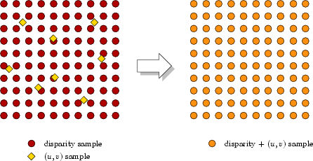 |
After verification, we are left with a set of reliable features, and a dense, regularly sampled disparity map, as shown in Figure 5.5. We would like to construct a unified representation that contains both 3D and parametric data, sampled in the same pattern. We choose to interpolate the parametric information given by the features to construct a dense, regularly sampled parametric map corresponding directly to the disparity map.
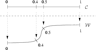
An interpolation in capture space is not sufficient, as demonstrated in Figures 5.6 and 5.7. As can be seen, linear interpolation in capture space leads to unacceptable distortions on the surface in world space. Instead, what is needed is linear interpolation along the surface (the arc in Figure 5.6). This must be extended from the one-dimensional example in the figure to a surface.
 |
This problem is similar in principle to the non-distorted texture mapping problem described by Lévy and Mallet [69] and others. Their technique enforced two primary constraints, perpendicularity and constant spacing of isoparametric curves on the surface. These goals are unfortunately not the same as our own: we desire constant spacing of isoparametric curves, but we would like to allow non-perpendicularity. In the language of the cloth literature, little or no stretch is permitted, while shearing may take place. Our problem is therefore subtly distinct from many of the standard problems in non-distorted texture mapping or mesh parameterisation.
First and foremost, we aim to perform a pure interpolation, retaining the parameterisation at all feature points. We choose to operate on individual triangles within the capture space Delaunay triangulation of the feature points. Within each such triangle the goal, like Lévy & Mallet, is to have constant spacing of isoparametric curves. We make no guarantees of C1 or C2 continuity across triangles.
Our interpolation scheme is recursive, and operates on a triangle mesh in capture space, typically a Delaunay triangulation of the input features. Parameters are known at every vertex of the mesh. Each triangle represents a curved surface patch, with the shape of the patch defined by the underlying disparity map.
We recursively subdivide each triangle into four smaller triangles
using the standard 4-to-1 split, but with one slight
difference. Instead of inserting new vertices at the capture space
midpoint of each edge, we insert at the geodesic midpoint. In other
words, if the endpoints of an edge are given by c1 and c2, the
new vertex
![]() satisfies
satisfies
![]() (where
(where ![]() is the approximate geodesic
distance from Equation 5.4), but it does not in general
satisfy
is the approximate geodesic
distance from Equation 5.4), but it does not in general
satisfy
![]() . Since this point
lies midway
between the endpoints, its parametric position is the average of the
endpoints' parameters. We form four new triangles using the three
original vertices and the three new midpoint vertices, and proceed
recursively on the smaller triangles.
. Since this point
lies midway
between the endpoints, its parametric position is the average of the
endpoints' parameters. We form four new triangles using the three
original vertices and the three new midpoint vertices, and proceed
recursively on the smaller triangles.
The recursion stops when a triangle encloses exactly one disparity sample. At this point, the triangle can be treated as flat. To find the parameters at the disparity sample location, we associate barycentric co-ordinates with the sample location and linearly interpolate the parameters of the triangle's vertices.
This interpolation scheme still has several problems. It is possible that the
correct interpolation between two features in
![]() follows a slightly
curved path in
follows a slightly
curved path in
![]() , instead of the straight line path used in this
interpolation algorithm. The distortion caused by this approximation should
be relatively subtle. More importantly, folds should receive special treatment
during interpolation. In theory, it may be possible to make a reasonable guess
about the world-space position of occluded regions hidden by the fold,
but we leave this as future work.
, instead of the straight line path used in this
interpolation algorithm. The distortion caused by this approximation should
be relatively subtle. More importantly, folds should receive special treatment
during interpolation. In theory, it may be possible to make a reasonable guess
about the world-space position of occluded regions hidden by the fold,
but we leave this as future work.
The final issue in interpolation is finding an appropriate way to resist shearing. In our approach, shearing is not dealt with directly (as Lévy and Mallet did), but we are not certain that this is the best decision. Cloth permits shearing, but it does also resist it. Our scheme does not explicitly incorporate this behaviour. Any algorithm which does mix stretch and shear resistance will have to choose a means of balancing resistance to these two types of forces. It is hard to envision a suitable way of balancing stretching and shearing without some knowledge of the cloth material; we leave this as future work.
![\includegraphics[width=.35\linewidth]{ctry-ref-keyvis}](ctry-ref-keyvis.png)
![\includegraphics[width=.35\linewidth]{ctry-img-keyvis}](ctry-img-keyvis.png)
![\includegraphics[width=.48\linewidth]{nointerp}](nointerp.png)
![\includegraphics[width=.48\linewidth]{interp}](interp.png)