[ HTML | PDF (web) | PDF (print) ]

3. Cloth Simulation Experiments

As part of our investigation of cloth simulation parameters, we wrote a cloth simulator. We implemented the simulator described by Baraff and Witkin [6], and released the software publicly with the name Freecloth. In Section 3.1, we discuss some corrections to Baraff and Witkin's paper. Using this simulator, we investigated the influence of each of the simulator's parameters. Details of this are discussed in Section 3.2.

3.1 Cloth Simulator

For our experiments, we used a simulator based on the approach of Baraff and Witkin. However, we modified their approach to include corrections made by other researchers, as well as improvements based on our own insights. Our implementation of Baraff and Witkin's algorithm included Ascher and Boxerman's corrections [4] to the modified preconditioned conjugate gradient algorithm, as well as their improved preconditioner.

Bhat et al. [11] noted issues with Baraff and Witkin's air drag formulation, and suggested corrections. We did not implement these corrections to air drag in our own cloth simulator. They also observed problems with excessive damping using the first-order implicit Euler time integration scheme used by Baraff and Witkin.

We note here a few corrections of our own. In particular, Baraff and Witkin's parameters are not scale-invariant. If a mesh is subdivided while all parameters are kept constant, the shape of the cloth changes substantially, beyond what would be expected through the simple introduction of a few edges for bending.

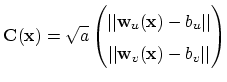
Baraff and Witkin defined forces in terms of what they called condition functions (C), which are closely related to energy (E):

$$E = \frac{k}{2} \mathbf{C}^T\mathbf{C}$$ (3.1)

They defined separate energies for stretching, shearing and bending. They presented a correct argument for keeping the bend condition function independent of triangle area, but defined the stretch and shear condition functions to be directly proportional to triangle area. Consequently, the stretch and shear energies are proportional to the square of the triangle area. If a triangle is refined in a standard 1-to-4 split, the total energy of the four new triangles will be one quarter of the original energy. Since bend and gravity energies are independent of tessellation, this makes stretch and shear forces relatively weak at higher tessellations, and dramatically changes the shape of the cloth drape as the cloth is refined.

We recommend modifying Baraff and Witkin's condition functions to be proportional to the square root of the triangle area, making the energies directly proportional to triangle area. The stretch condition function in Baraff and Witkin's equation (10) should be changed to use the square-root of the area,

$$\mathbf{C}(\mathbf{x}) = \sqrt{a} \begin{pmatrix} \lvert\lvert\ma... ...\rvert \\ \lvert\lvert\mathbf{w}_v(\mathbf{x})-b_v\rvert\rvert \end{pmatrix}$$

and the shear condition in section 4.3 of their paper should be likewise be changed,

$$C(\mathbf{x}) = \sqrt{a} \mathbf{w}_u(\mathbf{x})^T \mathbf{w}_v(\mathbf{x}).$$

This will make the cloth simulation parameters independent of mesh tessellation. Bhat et al. independently made the same observation.

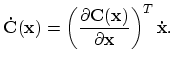
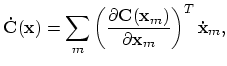
Finally, in equation (11) of Baraff and Witkin's paper, damping forces are calculated using $\mathbf{\dot{C}}(\mathbf{x})$, which they defined as

$$\mathbf{\dot{C}}(\mathbf{x}) = \left(\frac{\partial\mathbf{C}(\mathbf{x})}{\partial\mathbf{x}}\right)^T \mathbf{\dot{x}}.$$

Correct partial differentiation of $\mathbf{\dot{C}}(\mathbf{x})$ should give

$$\mathbf{\dot{C}}(\mathbf{x}) = \sum_m \left(\frac{\partial\mathbf{C}(\mathbf{x}_m)}{\partial\mathbf{x}_m}\right)^T \mathbf{\dot{x}}_m,$$

where m ranges over all particles influencing C. This was likely the authors' intent, but it is unclear (and even a little misleading) in their paper.

3.2 Influence of Parameters

For some cloth simulation algorithms [17], the relationship between the simulator's parameters and the mechanical behaviour of real cloth has been well-established. However, Baraff and Witkin's simulator has not been subjected to such study, and it is not intuitively obvious how the simulator's parameters affect cloth motion, or how they interact. We set out to investigate the effect of the individual parameters on cloth movement.

Bhat et al. [11] are the only authors to present plausible parameter values for Baraff and Witkin's cloth simulator. The base values used in our simulation are shown in Table 3.1. Bhat et al. used a different drag model, and did not use the MPCG algorithm or adaptive time stepping requiring a stretch limit. They did report stretch, shear and bend resistances and damping parameters that were within an order of magnitude of the parameters we used.

Table 3.1: Parameter values for the modified scale invariant version of Baraff and Witkin's simulator.

Parameter	Symbol	Value
Stretch resistance	kst	100
Shear resistance	ksh	10
Bend resistance	kb	1.0 × 10-5
Stretch damping	dst	20
Shear damping	dsh	2
Bend damping	db	2.0 × 10-6
Air drag	ka	0.1
MPCG tolerance		0.01
stretch limit		5.0 × 10-5

To evaluate the influence of the individual parameters, a series of simulations was performed. The setup involved the draping of a tablecloth over a circular table. The cloth was modelled as a square sheet of 66×66 square patches with a regular split into triangles. In each experiment, only a single parameter was varied, and a number of statistics were recorded, including the appearance of the cloth and the spatial distribution of stretch, shear and bend energy in the cloth. In the results that follow, spatial energy distributions are visualised by encoding the logarithm of the stretch, shear and bend energies in the red, green and blue channels of the image respectively, as shown in Figure 3.1.

Figure 3.1: Stretch, shear and bend energies are combined as the red, green and blue channels of a single image to visualise the overall energy distribution during cloth simulation.

(a) Stretch energy		(b) Shear energy		(c) Bend energy		(d) Combined

The experiments were limited to a single drape configuration, and only one parameter was changed at a time. Consequently, we can draw few substantial conclusions about the general behaviour of Baraff & Witkin's cloth model; we limit this section to our observations.

3.2.1 Number of patches

The effect of changing the discretisation of the cloth surface is demonstrated in Figure 3.2. In this particular tablecloth example, it appears that 66×66 patches is a sufficiently fine discretisation for a reasonable simulation. Both the final drape and the energy profile are very similar for the 66×66 case and the much finer 132×132 example.

Figure 3.2: Impact of discretisation on tablecloth drape and energy distribution.

patches	drape (2.4 s)		energy (2.4 s)		total energy
22×22
33×33
66×66
99×99
132×132

It is interesting to observe the changing energy profile in lower tessellation examples. When the surface was discretised coarsely, the cloth was very limited in its ability to bend, and was consequently forced to shear substantially. With finer discretisations, bending rose slightly and shearing dropped dramatically. The only real difference between the finest discretisations was a slight change in bending behaviour.

Clearly, the appropriate level of discretisation is highly application-dependent. A discretisation of 66×66 was sufficient for this tablecloth, but might be a poor choice for a complicated piece of clothing with finer wrinkles and many regions of high curvature.

3.2.2 Timestep

Figure 3.3: Impact of timestep on drape and energy distribution.

h	drape (0.4 s)		energy (0.4 s)		total energy
0.001
0.002
0.005
0.010
0.020

Large timesteps are known to introduce numerical damping, as demonstrated here. In this experiment a fixed timestep was used, and the damping impact can be seen in the mid-swing pose of the cloth shown in Figure 3.3 and also in the energy graph. Baraff and Witkin's goal of using large timesteps will clearly also force the cloth motion to be damped.

In terms of cloth parameter recovery, this result is quite significant. It implies that cloth parameters can only be reused in other simulations operating at the same timescale--if at all. Clearly, this behaviour needs further study if cloth parameter recovery is to be practical.

When using adaptive timestepping, varying amounts of damping were introduced into the system as the timestep grew and shrank, making it difficult to compare results between different trials. To reduce the effect of this behaviour, timesteps were kept small (5 ms) in the experiments that follow.

3.2.3 Stretch, shear and bend resistance

The effect of changing the cloth's resistance to stretch, shear and bend is demonstrated in Figures 3.4-3.6.

Figure 3.4: Impact of stretch resistance on energy distribution.

kst	energy (2.4 s)		total energy
20
50
100
200
1000

Changes to the stretch resistance had little effect on the movement of the cloth. The final drape and the transient motion were essentially unaffected over a wide range of values, although the total stretch energy stored in the cloth did change. With higher stretch resistance, stretch energy reached equilibrium rapidly, and less stretch energy was stored in the cloth in the transient régime.

Figure 3.5: Impact of shear resistance on drape and energy distribution.

ksh	drape (2.4 s)		energy (2.4 s)		total energy
1
10
50

Modifying the cloth's shear resistance had a more visible effect. With low shear resistance, the cloth's final drape showed more sag, and the shearing was quite evident in the cloth texture. When shear resistance was low, more shear energy was stored in the cloth and the cloth swung freely. When the shear resistance was higher, the cloth motion appeared highly damped.

Figure 3.6: Impact of bend resistance on drape and energy distribution.

kb	drape (2.4 s)		energy (2.4 s)		total energy
1 × 10-6
1 × 10-5
1 × 10-4

Changes to bend resistance obviously influenced the cloth's shape. With high bend resistance, relatively few wrinkles formed, and the bends that did form stored a large amount of bend energy.

3.2.4 Damping constants

From our observations of both real and simulated cloth, the only aspect of cloth motion that was visibly damped was bending. Both stretching and shearing behaviour seemed to be overdamped, while bending behaviour was either underdamped or overdamped, depending on the cloth material.

In the tablecloth draping experiments, the cloth either settled slowly on the table or else fell quickly onto the table and swung back and forth several times before settling to a steady state. This corresponded to overdamped and underdamped behaviour, respectively. In the energy graphs, this can generally be seen by looking for ringing behaviour in the total bend energy.

Figure 3.7: Impact of stretch damping constant on energy distribution.

dst	energy (0.32 s)		total energy
10
20
100

The impact of the stretch damping constant was fairly minimal. Subtle damping in the motion of the cloth was evident during the first second of movement, but the final drape was unaffected. As shown in Figure 3.7, the energy graph shows changes to the transient energy distribution, with obvious damping effects in the stretch energy as the damping constant rose. Curiously, with very low stretch damping (e.g., $d_{st} \leq 2$), the simulation could not be computed.

Figure 3.8: Impact of shear damping constant on energy distribution.

dsh	energy (0.08 s)		total energy
0.02
2.00
4.00

The shear damping constant also had only a minor effect on the cloth's behaviour. The cloth's final drape and motion were unaffected by changes to this constant. The energy graph shows predictable underdamped and critically damped behaviour in the shear energy, but the transient behaviour was brief enough that it had no major effect on the cloth's motion. Figure 3.8 shows the cloth energy distribution near the beginning of the simulation.

Figure 3.9: Impact of bend damping constant on energy distribution.

db	energy (0.16 s)		energy (0.52 s)		total energy
2 × 10-7
2 × 10-6
1 × 10-5

The bend damping constant had a very visible effect on the cloth's movement. As shown in the energy graphs in Figure 3.9, the bend energy was quite different as the constant was changed, and this could also be seen in the cloth's movement, particularly at the corners. The damping was predictable and followed a typical underdamped/overdamped form, but there was also some interesting smoothing. When the bending damping constant was low, fine wrinkles formed in the cloth during the early transient motion, while damping prevented these wrinkles from forming when the bending damping constant was higher. The final drape position was the same in all cases, however.