Next: 4 Verification Up: Implementing Baraff & Witkin's Previous: 2 Notation
Baraff & Witkin used condition functions as an indirect way of defining
energy and forces. Their condition functions are almost the same as energy
formulas, since
![]() , where
, where ![]() is the
condition function. For the scalar condition functions (shear and bend),
is the
condition function. For the scalar condition functions (shear and bend),
![]() , and the condition function is hence basically just the
squart-root of the energy, except that it can be positive or negative.
, and the condition function is hence basically just the
squart-root of the energy, except that it can be positive or negative.
The condition functions were defined explicitly in the paper. Energy and forces can also be easily calculated, if the derivatives of the condition functions are known. However, the paper didn't provide explicit equations for the derivatives or second derivatives.
Macri made a good attempt at deriving the equations for the derivatives and second derivatives. I found two major shortcomings in his approach, however. First, he made reference to tensors and other mathematical constructs that aren't really necessary for the derivation. Second, I found an error in his derivation for the bend condition.
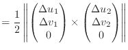
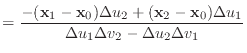
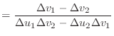
To begin, I will define a few quantities that will help with explanation of
the stretch and shear conditions. These quantities are defined for a triangle
using points ![]() ,
, ![]() , and
, and ![]() . The triangle's area in
. The triangle's area in ![]() /
/![]() space
is given by
space
is given by
 |
(1) |
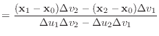
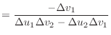
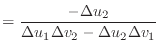
The
![]() and
and
![]() vectors represent the directions of the
vectors represent the directions of the ![]() and
and ![]() axes in world space, as seen within a single triangle. They are defined by
axes in world space, as seen within a single triangle. They are defined by
| (2) |
 |
(3) | |
 |
(4) |
The first derivatives of the unnormalised vectors ![]() and
and ![]() are
given by
are
given by
 |
(5) | |
 |
(6) | |
 |
(7) | |
 |
(8) |
 |
(9) | |
 |
(10) | |
 |
(11) | |
 |
(12) |
The second derivatives of ![]() and
and ![]() are all zero.
are all zero.
Baraff & Witkin define the stretch condition function as a vector ![]() .
Two special parameters are defined for stretch,
.
Two special parameters are defined for stretch, ![]() and
and ![]() . These
represent the desired stretchiness of the cloth in the
. These
represent the desired stretchiness of the cloth in the ![]() and
and ![]() directions.
A
directions.
A ![]() value below one will result in the cloth trying to compress in the
value below one will result in the cloth trying to compress in the ![]() direction, while a
direction, while a ![]() value above one will result in the cloth trying to
stretch in the
value above one will result in the cloth trying to
stretch in the ![]() direction.
direction.
 |
 |
(13) |
Baraff & Witkin defined ![]() , the area of the triangle. We define
, the area of the triangle. We define
![]() , for reasons described later.
, for reasons described later.
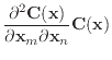
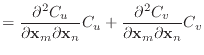
The first and second derivatives of the stretch condition function are
 |
(14) | |
 |
 |
(15) |
 |
(16) | |
 |
 |
(17) |
These second derivatives exhibit some symmetry, since
![]() .
Consequently, the
.
Consequently, the ![]() matrix
matrix
![]() .
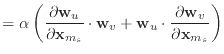
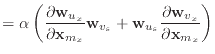
To avoid any tensors when applying Baraff & Witkin's equation (8) to the
shear equations, remember that
.
To avoid any tensors when applying Baraff & Witkin's equation (8) to the
shear equations, remember that
 |
 |
(18) |
Baraff & Witkin define the shear condition function as a scalar. This
scalar is essentially the dot product of the ![]() axis with the
axis with the ![]() axis in
world space. If no shear is occurring, the axes are perpendicular and the
condition function is zero. If shear is occurring, the condition function is
equivalent to the cosine of the angle between them, weighted by the triangle's
area in
axis in
world space. If no shear is occurring, the axes are perpendicular and the
condition function is zero. If shear is occurring, the condition function is
equivalent to the cosine of the angle between them, weighted by the triangle's
area in ![]() /
/ ![]() space.
space.
Baraff & Witkin's condition assumes that ![]() and
and ![]() are approximately
unit vectors. If
are approximately
unit vectors. If ![]() and
and ![]() are both equal to one, then this approximation
is a fair one. If, however,
are both equal to one, then this approximation
is a fair one. If, however, ![]() or
or ![]() are not equal to one, the
approximation may give rise to some strange behaviour. I have not had a chance
to investigate the effects of varying
are not equal to one, the
approximation may give rise to some strange behaviour. I have not had a chance
to investigate the effects of varying ![]() or
or ![]() .
.
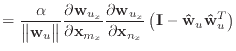
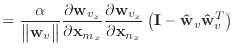
Since we know the derivatives of ![]() and
and ![]() , taking the derivative of
this condition function is trivial.
, taking the derivative of
this condition function is trivial.
 |
(20) | |
 |
(21) |
 |
||
 |
||
 |
(22) | |
| (23) |
These second derivatives exhibit even more symmetry than the stretch
condition. Like the stretch condition,
![]() but beyond that, the
but beyond that, the
![]() is actually just an identity matrix multiplied by a
scalar.
is actually just an identity matrix multiplied by a
scalar.
Baraff & Witkin define the bend condition in terms of two adjoining triangles.
I have labelled the unit normals of these triangles as
![]() and
and
![]() ,
rather than Baraff & Witkin's
,
rather than Baraff & Witkin's ![]() or
or ![]() . The unit vector
parallel to their common edge is labelled
. The unit vector
parallel to their common edge is labelled
![]() . Quantities associated with
the normals or the common edge receive a superscript
. Quantities associated with
the normals or the common edge receive a superscript ![]() ,
, ![]() or
or ![]() .
.
 |
 |
(24) |
| (25) | ||
| (26) | ||
| (27) |
The scalar bend condition ![]() is defined quite simply as the angle between
the two edges,
is defined quite simply as the angle between
the two edges, ![]() .
.
Macri defined ![]() using the
using the ![]() function, which is incorrect and will
only yield positive values for
function, which is incorrect and will
only yield positive values for ![]() . My definition of
. My definition of ![]() will yield
both positive and negative values if implemented using the atan2 function.
will yield
both positive and negative values if implemented using the atan2 function.
In order to find the derivatives of ![]() , we need the derivatives
of the quantities seen so far. The first and second derivatives of
, we need the derivatives
of the quantities seen so far. The first and second derivatives of
![]() ,
, ![]() and
and ![]() are shown below, using auxiliary variables
are shown below, using auxiliary variables
![]() . The derivatives of
. The derivatives of ![]() are straightforward to derive.
are straightforward to derive.
| (31) | ||
| (32) | ||
| (33) |
| (34) | ||
| (35) | ||
| (36) |
 |
 |
(37) |
 |
 |
(38) |
 |
(39) |
Using Baraff & Witkin's assumption that the normal and edge vectors have constant magnitude,
 |
(40) | |
 |
(41) | |
 |
(42) |
 |
 |
(43) |
 |
 |
(44) |
 |
(45) |
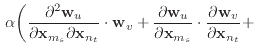
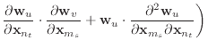
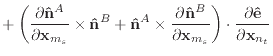
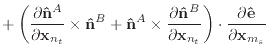
Given the derivatives of the normal and edge vectors, the first and second
derivatives of
![]() and
and
![]() are trivial to calculate.
are trivial to calculate.
 |
 |
(46) |
 |
(47) |
 |
 |
(48) |
 |
||
 |
(49) |
 |
 |
|
 |
(50) |
 |
||
 |
||
 |
||
 |
||
 |
||
 |
(51) |
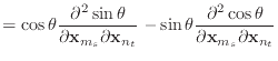
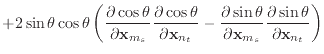
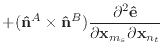
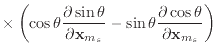
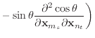
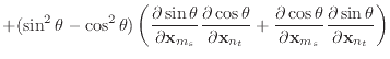
Finally, we can differentiate equation (30) to obtain the
derivatives of ![]() .
.
 |
(52) | |
 |
(53) | |
 |
(54) |
In a manner similar to the stretch condition,
![]() and the
and the ![]() matrix is symmetric. The
second derivatives of
matrix is symmetric. The
second derivatives of
![]() and
and
![]() are likewise symmetric.
are likewise symmetric.
![$\displaystyle + 2 \sin\theta \cos\theta \left( \frac{\partial \cos \theta}{\par...
...bf x}_{m_s}} \frac{\partial \sin \theta}{\partial {\bf x}_{n_t}} \right) \Bigg]$](img189.png)