David Pritchard
Department of Computer Science
University of British Columbia
Techniques for cloth simulation have advanced greatly over the past few years. Faster simulation algorithms [1], resolution of friction and collision detection [4], and methods of dealing with wrinkles and buckling [5] have advanced the state of the art.
To date, however, there have been few efforts to measure the movement of real cloth. Such measurements could be used to infer parameters for a specific material type, or to verify the correctness of cloth simulators. Many authors fall back upon the old computer graphics adage, ``if it looks right, it is right'' [7]. Breen et al. [3] and Eberhardt et al. [6] have incorporated data from the Kawabata measurement system into their cloth simulation systems, but there is as yet no way to use Kawabata data with more modern simulators. Furthermore, the Kawabata device is expensive and special-purpose. It would be more convenient to be able to determine parameters for simulation systems using conventional equipment such as video capture devices. Furthermore, video allows more information to be obtained about cloth movement.
In this paper, I present a technique for recovering information about the position and deformation of a sheet of rectangular cloth with a printed grid pattern. The cloth is first acquired using a Digiclops camera and stereo correspondence, producing a colour image and a depth map. Subsequently, deformation of the cloth is measured by detecting features in the grid pattern.
The most similar work to mine is that of Jojic et al. [8], who tried to estimate cloth draping parameters from range data. Their technique used only range data without associated colour information. They treated the range data as a solid surface, and used a cloth simulator to drape an imaginary cloth over the solid surface, from which they inferred cloth parameters. Many details of this technique remain unclear.
Louchet et al. [9] used synthetic data from a simulation to recover dynamic parameters for a mass-spring based cloth simulator. The input to their system is not specified explicitly, but it was not images; instead, a 3D mesh of cloth points was likely used. Their work does not, then, overlap with my own.
A number of algorithms were considered for recovery of depth from images. For the purposes of this project, the ideal algorithm would:
Of the available shape recovery algorithms, stereo correspondence comes the closest to meeting these requirements. Correspondence algorithms require textured cloth--not necessarily large-scale patterns, but certainly fine-scale texture, in the form of visible strands or fluff. This limits the range of materials that can be captured; in my tests, cotton T-shirts were often unacceptable, but fluffy teatowels worked quite well. Fine texture could be added in other acceptable ways, however, such as a light spray-paint layer. Stereo correspondence is a passive technique, allows capture of any surface type, and is easy to implement. Its precision is limited, since depth samples are quantised by the capture process.
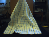
Capture was performed using a Digiclops camera, manufactured by Point Grey Research. Due to limited dynamic range, lighting had to be carefully controlled. Incandescent light produced good results, but indirect natural light seemed did an even better job at depth recovery. White cloth was found to be easier to capture than darker shades. The cloth was suspended by one edge from a stand, and placed against a dark background for easy segmentation. The cloth used was a white cotton teatowel with printed blue and yellow stripes. The vertical stripes were solid, while the horizontal stripes were a mixture of colour and white stitching.
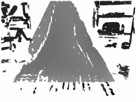
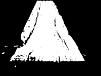
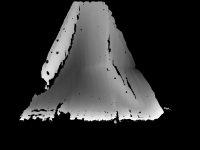
The Digiclops provided three images (right, top and left), each at 1024x768. Stereo processing was performed on greyscale images using the Triclops SDK. Images were rectified, low-pass filtered, and edge-filtered. Stereo correspondence was performed on the images, and points were validated using a median filter. The full list of parameters used is shown in Table 1. After processing with the Triclops SDK, the final output of the capture process was a colour image, a depthmap, and a mask indicating the valid pixels. All outputs are shown from the right camera's view in Figure 1.
 |
 |
 |
 |
Subpixel interpolation was used, but had some definite disadvantages. Stereo correspondence algorithms are limited to a maximum precision of one pixel. This leads to quantisation of the depth data, yielding a coarse, jagged appearance. Subpixel interpolation attempts to solve this problem by interpolating depth values to produce a smoother surface. Unfortunately, high contrast edges of the cloth gave rise to errors in the interpolated depth data, as seen in Figure 2. These ridges are not present in the actual geometry of the cloth. A flat sheet of paper with a checkerboard pattern produced similar artefacts.
![\begin{figure}\centering\includegraphics[width=4cm]{quantc}
\includegraphics[width=4cm]{quantd}
\end{figure}](img6.png) |
For the purposes of this paper, these ridges are accepted as a source of error. For more accurate results, they should be filtered out, or some other technique should be used to deal with quantisation errors. It remains uncertain whether the errors are caused by subpixel interpolation, or if they were already present in the data and were simply more obvious after interpolation.
The acquisition process produced three images: a colour image, a depth image, and a binary mask specifying which parts of the images contain valid data. These images contain information about both the cloth and the backdrop.
Colour and depth data contains some useful information about the properties of the underlying cloth. However, to understand the material properties and dynamic behaviour of cloth, more information is needed about the cloth surface. Topological information is needed in order to recover the shape of the cloth and to help with the identification of folds and wrinkles in the surface. Measurements of the surface deformation--stretch, shear and bend--can help with understanding the physical properties of the cloth material.
Recovering this information from the acquired data is a nontrivial task. To fully recover topology requires knowledge of sections of the cloth which may be occluded in the depth buffer by folds in the cloth. Measuring the exact stretch, shear or bend of the surface at any point is also a difficult task. To simplify the extraction of topology and deformation, a few simplifying assumptions were made. The cloth was assumed to be rectangular, with a grid pattern printed on it. By identifying the grid intersection points, a rough estimate of the cloth topology was established. Furthermore, by examining the distortion of the rectangles defined by the grid, the local surface deformation could also be estimated.
A similar approach has been used in cloth simulation. Baraff and Witkin [1] discretised a cloth surface into a triangular mesh, then measured the stretch and shear energy in each triangle, and the bend energy between pairs of triangles. These energies were used to determine forces to apply to the mesh vertices. In their paper, they consider the position of each mesh vertices in a flat, undeformed mesh in the (u,v) plane. Each vertex thus had two sets of co-ordinates: (u,v) co-ordinates defining its undeformed position, and (x,y,z) co-ordinates defining its actual position in three-dimensional space. Baraff and Witkin defined energy functions to measure stretching, shearing and bending in the cloth using this information.
I have adopted Baraff and Witkin's convention for co-ordinates. In this section, I summarise a technique for detecting grid vertices, and for then recovering (u,v) information.
The grid pattern printed on the cloth had two overlaid grids, one in blue and one in yellow, printed on top of a white cloth. The yellow grid had poor contrast against the white background, so only the blue grid was used for extraction. This was accomplished by using only the red channel of the acquired colour image.
The grid vertex detection scheme depends upon two inputs: the red channel of the colour image, and a mask defining the valid regions in the image. The grid vertices were difficult to detect with conventional schemes, such as the SUSAN corner detector [13]. Instead, greyscale mathematical morphology techniques were used [10],[12]. MATLAB was used for all of these image-processing operations.
The overall strategy was to detect the squares bounded by the grid. For each square, the set of neighbouring squares was established. Using these neighbours, the set of squares bounding each corner could be determined. Finally, the corners were detected by finding the point that was minimally distant from each square.
In a first pass, the squares bounded by the grid are detected using the watershed transform introduced by Beucher [2]. The intuitive explanation for this transform involves picturing the image as a heightfield, where intensity represents height. In this terrain, there are a number of catchment basins (local minima). If one imagines slowly rising water emerging from the bottom of each basin, eventually the water will reach a stage where two catchment basins merge. The points where the basins merge form ``watershed lines''. The watershed transform uses this analogy to label each independent catchment basin in the input image, and to identify all watershed lines.
For the detection of grid points, the squares bounded by the grid were treated as catchment basins, and the grid lines are the watershed. The image was inverted, so that the white squares became valleys and the dark grid lines became peaks. Contrast enhancement was used to amplify the difference between peaks and valleys. Using a thresholding operation (the extended-minima transform), most of the valleys were forced to zero. Finally, the watershed transformation was applied. The combination of the extended-minima operation and the watershed transformation is equivalent to a watershed-from-markers operation.
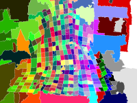
The watershed transform labels pixels in each catchment basin with a unique value, as shown in Figure 3. There are a number of incorrect small basins, typically caused by aliasing artefacts near the two thick vertical stripes. By calculating the area of each catchment basin and rejecting basins below a minimum size, these can be eliminated. A dilated version of the mask was used to eliminate basins outside the mask.
 |
 |
Some errors are evident: adjacent squares were sometimes merged, and individual squares were sometimes split. By adjusting the threshold used in the extended-minima transform, it was possible to prefer more merging errors and less splitting errors, or the opposite. In the end, splitting errors were found to be preferable to merging errors.
To find the neighbours of a given square, the following procedure was used. The watershed image provided a mask for the square, indicating all pixels belonging to the square. A residue mask was constructed by dilating the square mask with a two-pixel radius disc, and then subtracting the square mask. This residue mask was in turn used with the watershed image to find the neighbouring squares, as demonstrated in Figure 4. Neighbours with many pixels in the dilated mask shared an edge, and were part of the 4-neighbourhood of this square. Neighbours with only a few pixels in the dilated mask probably share a corner with this square, but not an edge, and were hence part of the 8-neighbourhood of the square. The process was repeated with a larger-radius disk for the mask dilation, to find all of the 8-neighbours of the square. For better performance, all of these operations were performed on a cropped image.
 |
 |
 |
 |
The corner detector takes a list of squares ![]() as input, and finds the
point which is ``closest'' to all four squares. To be precise, it finds the
point
as input, and finds the
point which is ``closest'' to all four squares. To be precise, it finds the
point ![]() that minimises
that minimises
 |
 |
 |
 |
 |
To obtain the list of squares for input to the corner detection routine, a slightly ad hoc strategy was necessary. First, a set of four squares was tried: a reference square, two of its 4-neighbours, and one diagonal 8-neighbour. By using a radial sort of the neighbours, these squares were guaranteed to share a corner. If this failed due to a missing neighbour, it was retried with two 4-neighbours, or one 4-neighbour and an 8-neighbour. If only a single 4-neighbour was available, no corner was measured.
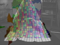
The final set of corners is shown in Figure 6. As can be seen, there are a number of incorrect corners. These are mostly due to the choice of threshold in the watershed stage. By preferring splitting to merging, less false negatives are obtained, but more false positives are generated. Even still, there are a handful of corners that were not detected. There are a number of techniques that could remedy this: repeated attempts with different thresholds in the watershed stage could help, as could detection of corners in the case where only a 4-neighbour was available.
In order to associate a (u,v) co-ordinate with each of these points, user interaction was required. The user was shown a point and asked to enter its position on the grid (an integer number of squares from the bottom left corner), which was then mapped to a (u,v) value in the unit square. The user was also able to reject incorrect corners.
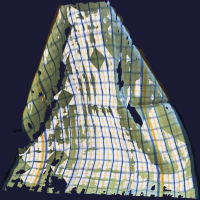
In order to evaluate the quality of the measurements, two meshes were constructed. The first mesh was built using the data acquired during the acquisition stage, using a heightfield to represent the acquired depth map, and applying the colour image as a texture on this heightfield. Since the source depth map is large (1024x768), this mesh has a lot of fine detail.
The second mesh was built using the detected grid vertices. A depth value was determined for each grid vertex by doing a lookup in the depth map. For a texture, a scan of the flattened cloth was used. The grid has only a small number of vertices (21x25), so this mesh is quite coarse.
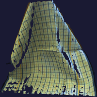
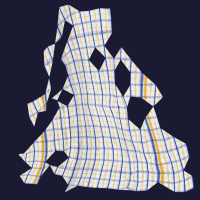
These two meshes are shown in Figure 7, along with a superimposition of the two. The colours in the two meshes are different, since the first mesh was acquired using a careful lighting setup to allow good depth measurement, while the second mesh's texture is simply a scan of the cloth. As can be seen in the superimposition, the grid lines match up quite well between the two meshes, indicating a good measurement of the grid vertex positions.
While capture was successful over the large, mostly flat regions of the cloth, there were problems in the large fold in the top left corner. Here, only sparse data was able to be captured. There are also patches of cloth that are missing, some of which were due to creases that were mistaken for grid intersections.
 |
 |
 |
Samaras et al. [11] describe an improved stereo algorithm incorporating shape-from-shading that works with surfaces of variable albedo. This technique might prove useful for improving the depth data acquisition.
In this work, (u,v) co-ordinates were only measured for the grid vertices. However, interpolated (u,v) co-ordinates could be used for all other depth samples, giving a complete depth map with (u,v) information. In this case, the (u,v) co-ordinates would be more unreliable, since minor features such as wrinkles and creases would not be accounted for; however, the finer geometry might still be useful.
Using the (u,v) values found here, one could also measure actual stretch, shear and bend distributions over the cloth. It may also be possible to infer the most likely parameters for a given cloth simulator given this data and a suitable experimental setup.
This work was supported in part by a scholarship from the Natural Sciences and Engineering Research Council of Canada, and by the British Columbia Advanced Systems Institute.