David Pritchard
Date: May 2003, with minor updates April 2012
In April 2002, I implemented a cloth simulator based on Baraff & Witkin's paper [BW98] for a graduate animation course taught by Michiel van de Panne at the University of British Columbia. I later released that simulator as an open-source project called Freecloth. Over the following year, I improved the performance of the simulator and fixed some major bugs.
The initial version of Freecloth had some major bugs, and did not implement all parts of the original paper. Newer versions have eliminated the bugs in the simulator, but do not yet include all parts of the original paper.
I will assume that you are familiar with Baraff & Witkin's paper, and I will not try to re-explain concepts which are clearly presented there. For my own work, I relied heavily upon a paper by Dean Macri [Mac00], who attempted to interpret and implement Baraff & Witkin's paper. I will make reference to Macri's notation and some of his formulas, but his paper is not necessary reading. I rederived all of the formulas found in Macri's paper, and verified my derivation against Macri's. Initially, I found a few minor typographical errors in his paper, but my formulas were generally the same.
As my implementation progressed, I found more major errors in Macri's paper. The largest error occurred when he calculated the derivatives of the bend condition. I give a corrected version of this equation in (54) and (57).
In this paper, I will attempt to explain obstacles that I encountered while implementing Baraff & Witkin's paper.
In this paper, I will use the symbol ![]() to denote an identity matrix. The
symbol
to denote an identity matrix. The
symbol ![]() refers to a vector containing the
refers to a vector containing the ![]() th column of the identity
matrix. To
denote the skew-symmetric matrix form of a vector cross product, I will use
the notation
th column of the identity
matrix. To
denote the skew-symmetric matrix form of a vector cross product, I will use
the notation
I will also define the vector
![]() as the transpose of the
as the transpose of the
![]() th row of
th row of
![]() .
. ![]() is a column vector, but represents
a row in the original
is a column vector, but represents
a row in the original ![]() matrix.
I will use a hat (e.g.
matrix.
I will use a hat (e.g.
![]() ) to refer to a normalised vector of unit
length, and omit the hat (e.g.
) to refer to a normalised vector of unit
length, and omit the hat (e.g. ![]() ) for an unnormalised vector. This is
the opposite convention to that used in my original project report.
) for an unnormalised vector. This is
the opposite convention to that used in my original project report.
I will retain Baraff & Witkin's notation and use ![]() to refer to the
positions of points, not
to refer to the
positions of points, not ![]() as in Macri's paper. Furthermore,
I will refer to the points of a triangle as
as in Macri's paper. Furthermore,
I will refer to the points of a triangle as ![]() ,
, ![]() and
and ![]() , and
not use the
, and
not use the ![]() ,
, ![]() and
and ![]() subscripts used by the other two papers. For
the points of an edge, I will likewise use subscripts of 0, 1, 2, and 3 rather
than the
subscripts used by the other two papers. For
the points of an edge, I will likewise use subscripts of 0, 1, 2, and 3 rather
than the ![]() ,
, ![]() ,
, ![]() and
and ![]() subscripts used by Macri.
subscripts used by Macri.
When referring to points, I will use ![]() and
and ![]() to refer to two
possibly distinct points. I will use the subscript
to refer to two
possibly distinct points. I will use the subscript ![]() to refer to the
to the
to refer to the
to the ![]() th component of
th component of ![]() , and likewise the subscript
, and likewise the subscript ![]() for
the
for
the ![]() th component of
th component of ![]() . I will also sometimes use subsubscripts of
. I will also sometimes use subsubscripts of ![]() ,
,
![]() and
and ![]() to refer to the components.
to refer to the components.
I like to think of the derivatives in this paper in terms of their components. Both Baraff & Witkin and Macri differentiate with respect to a vector in their papers, giving quantities like
 |
 |
This type of formula is common in some areas of graphics; for example, the
Jacobian matrix has this form. However, what happens when we take the second
derivative of ![]() ? It will yield a third-order tensor, a
? It will yield a third-order tensor, a
![]() linear algebraic quantity. However, this is unnecessarily
complicated, especially for people (like me) who never covered tensors in
their undergraduate education. In this paper, I will try to avoid
differentiation with respect to a vector. Instead, I will do most of the work
on a component-by-component basis, using only differentiation with respect to
a scalar. Using this approach, I will only ever need to use vectors and
scalars, not matrices or higher-order tensors. This makes operations such as
cross-products and dot-products straightforward.
linear algebraic quantity. However, this is unnecessarily
complicated, especially for people (like me) who never covered tensors in
their undergraduate education. In this paper, I will try to avoid
differentiation with respect to a vector. Instead, I will do most of the work
on a component-by-component basis, using only differentiation with respect to
a scalar. Using this approach, I will only ever need to use vectors and
scalars, not matrices or higher-order tensors. This makes operations such as
cross-products and dot-products straightforward.
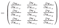
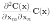
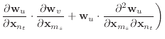
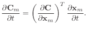
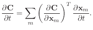
Some of Baraff & Witkin's formulas involve taking a second derivative with respect to two vectors. For these, just remember the layout of the resulting matrix. For example,
 |
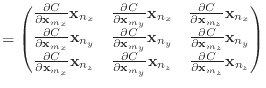 |
Baraff & Witkin used condition functions as an indirect way of defining
energy and forces. Their condition functions are almost the same as energy
formulas, since
![]() , where
, where ![]() is the
condition function. For the scalar condition functions (shear and bend),
is the
condition function. For the scalar condition functions (shear and bend),
![]() , and the condition function is hence basically just the
squart-root of the energy, except that it can be positive or negative.
, and the condition function is hence basically just the
squart-root of the energy, except that it can be positive or negative.
The condition functions were defined explicitly in the paper. Energy and forces can also be easily calculated, if the derivatives of the condition functions are known. However, the paper didn't provide explicit equations for the derivatives or second derivatives.
Macri made a good attempt at deriving the equations for the derivatives and second derivatives. I found two major shortcomings in his approach, however. First, he made reference to tensors and other mathematical constructs that aren't really necessary for the derivation. Second, I found an error in his derivation for the bend condition.
To begin, I will define a few quantities that will help with explanation of
the stretch and shear conditions. These quantities are defined for a triangle
using points ![]() ,
, ![]() , and
, and ![]() . The triangle's area in
. The triangle's area in ![]() /
/![]() space
is given by
space
is given by
 |
(1) |
The
![]() and
and
![]() vectors represent the directions of the
vectors represent the directions of the ![]() and
and ![]() axes in world space, as seen within a single triangle. They are defined by
axes in world space, as seen within a single triangle. They are defined by
| (2) |
 |
(3) | |
 |
(4) |
The first derivatives of the unnormalised vectors ![]() and
and ![]() are
given by
are
given by
 |
(5) | |
 |
(6) | |
 |
(7) | |
 |
(8) |
 |
(9) | |
 |
(10) | |
 |
(11) | |
 |
(12) |
The second derivatives of ![]() and
and ![]() are all zero.
are all zero.
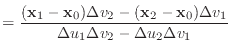
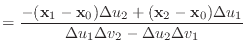
Baraff & Witkin define the stretch condition function as a vector ![]() .
Two special parameters are defined for stretch,
.
Two special parameters are defined for stretch, ![]() and
and ![]() . These
represent the desired stretchiness of the cloth in the
. These
represent the desired stretchiness of the cloth in the ![]() and
and ![]() directions.
A
directions.
A ![]() value below one will result in the cloth trying to compress in the
value below one will result in the cloth trying to compress in the ![]() direction, while a
direction, while a ![]() value above one will result in the cloth trying to
stretch in the
value above one will result in the cloth trying to
stretch in the ![]() direction.
direction.
 |
 |
(13) |
Baraff & Witkin defined ![]() , the area of the triangle. We define
, the area of the triangle. We define
![]() , for reasons described later.
, for reasons described later.
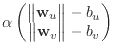
The first and second derivatives of the stretch condition function are
 |
(14) | |
 |
 |
(15) |
 |
(16) | |
 |
 |
(17) |
These second derivatives exhibit some symmetry, since
![]() .
Consequently, the
.
Consequently, the ![]() matrix
matrix
![]() .
To avoid any tensors when applying Baraff & Witkin's equation (8) to the
shear equations, remember that
.
To avoid any tensors when applying Baraff & Witkin's equation (8) to the
shear equations, remember that
 |
 |
(18) |
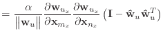
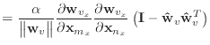
Baraff & Witkin define the shear condition function as a scalar. This
scalar is essentially the dot product of the ![]() axis with the
axis with the ![]() axis in
world space. If no shear is occurring, the axes are perpendicular and the
condition function is zero. If shear is occurring, the condition function is
equivalent to the cosine of the angle between them, weighted by the triangle's
area in
axis in
world space. If no shear is occurring, the axes are perpendicular and the
condition function is zero. If shear is occurring, the condition function is
equivalent to the cosine of the angle between them, weighted by the triangle's
area in ![]() /
/ ![]() space.
space.
Baraff & Witkin's condition assumes that ![]() and
and ![]() are approximately
unit vectors. If
are approximately
unit vectors. If ![]() and
and ![]() are both equal to one, then this approximation
is a fair one. If, however,
are both equal to one, then this approximation
is a fair one. If, however, ![]() or
or ![]() are not equal to one, the
approximation may give rise to some strange behaviour. I have not had a chance
to investigate the effects of varying
are not equal to one, the
approximation may give rise to some strange behaviour. I have not had a chance
to investigate the effects of varying ![]() or
or ![]() .
.
Since we know the derivatives of ![]() and
and ![]() , taking the derivative of
this condition function is trivial.
, taking the derivative of
this condition function is trivial.
 |
(20) | |
 |
(21) |
 |
||
 |
||
 |
(22) | |
| (23) |
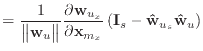
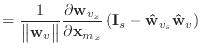
These second derivatives exhibit even more symmetry than the stretch
condition. Like the stretch condition,
![]() but beyond that, the
but beyond that, the
![]() is actually just an identity matrix multiplied by a
scalar.
is actually just an identity matrix multiplied by a
scalar.
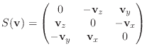
Baraff & Witkin define the bend condition in terms of two adjoining triangles.
I have labelled the unit normals of these triangles as
![]() and
and
![]() ,
rather than Baraff & Witkin's
,
rather than Baraff & Witkin's ![]() or
or ![]() . The unit vector
parallel to their common edge is labelled
. The unit vector
parallel to their common edge is labelled
![]() . Quantities associated with
the normals or the common edge receive a superscript
. Quantities associated with
the normals or the common edge receive a superscript ![]() ,
, ![]() or
or ![]() .
.
 |
 |
(24) |
| (25) | ||
| (26) | ||
| (27) |
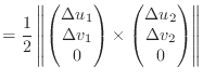
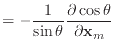
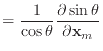
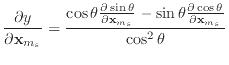
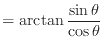
The scalar bend condition ![]() is defined quite simply as the angle between
the two edges,
is defined quite simply as the angle between
the two edges, ![]() .
.
Macri defined ![]() using the
using the ![]() function, which is incorrect and will
only yield positive values for
function, which is incorrect and will
only yield positive values for ![]() . My definition of
. My definition of ![]() will yield
both positive and negative values if implemented using the atan2 function.
will yield
both positive and negative values if implemented using the atan2 function.
In order to find the derivatives of ![]() , we need the derivatives
of the quantities seen so far. The first and second derivatives of
, we need the derivatives
of the quantities seen so far. The first and second derivatives of
![]() ,
, ![]() and
and ![]() are shown below, using auxiliary variables
are shown below, using auxiliary variables
![]() . The derivatives of
. The derivatives of ![]() are straightforward to derive.
are straightforward to derive.
| (31) | ||
| (32) | ||
| (33) |
| (34) | ||
| (35) | ||
| (36) |
 |
 |
(37) |
 |
 |
(38) |
 |
(39) |
Using Baraff & Witkin's assumption that the normal and edge vectors have constant magnitude,
 |
(40) | |
 |
(41) | |
 |
(42) |
 |
 |
(43) |
 |
 |
(44) |
 |
(45) |
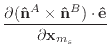
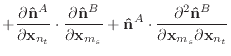
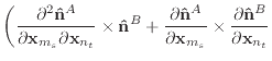
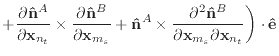
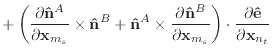
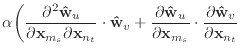
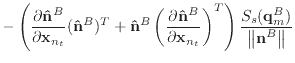
Given the derivatives of the normal and edge vectors, the first and second
derivatives of
![]() and
and
![]() are trivial to calculate.
are trivial to calculate.
 |
 |
(46) |
 |
(47) |
 |
 |
(48) |
 |
||
 |
(49) |
 |
 |
|
 |
(50) |
 |
||
 |
||
 |
||
 |
||
 |
||
 |
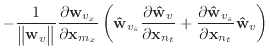
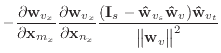
(51) |
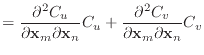
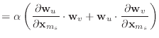
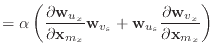
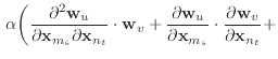
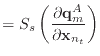
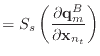
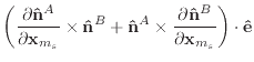
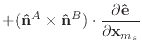
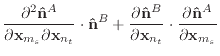
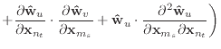
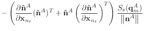
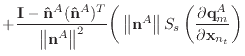
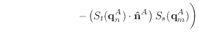
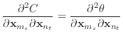
Finally, we can differentiate equation (30) to obtain the
derivatives of ![]() .
.
 |
(52) | |
 |
(53) | |
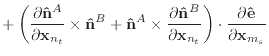
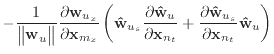
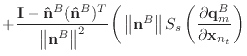
 |
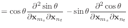
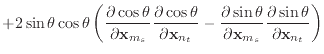
(54) |
In a manner similar to the stretch condition,
![]() and the
and the ![]() matrix is symmetric. The
second derivatives of
matrix is symmetric. The
second derivatives of
![]() and
and
![]() are likewise symmetric.
are likewise symmetric.
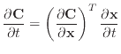
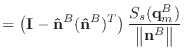
Macri didn't describe any way of verifying the correctness of his derivations or implementation. Once I had initially implemented the simulator, I found bugs but had no way of determining where an error was occurring. To address this, I used numeric derivatives.
For example, suppose that we need to verify the calculation of
![]() . Our program calculates the derivative using an analytic
formula, which we'll call
. Our program calculates the derivative using an analytic
formula, which we'll call ![]() . The derivative can also be calculated
numerically:
. The derivative can also be calculated
numerically:
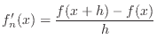
If
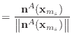
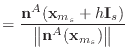
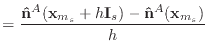
Verification is a little bit trickier for the bend condition. Here, we can't
just use a normal derivative, since we have to differentiate under the
assumption that the vectors have constant magnitude. Suppose that we want
to verify the derivative
![]() . Let
. Let
![]() represent
the normal with point
represent
the normal with point ![]() at position
at position
![]() , and
, and
![]() represent the normal once point
represent the normal once point ![]() 's
's ![]() th component is shifted by
th component is shifted by ![]() .
The unit normals are then given by
.
The unit normals are then given by
 |
||
 |
 |
To be honest, I don't know why numeric derivatives can't be used for everything. I suspect that they may be less robust than analytic derivatives, and there may be a performance tradeoff involved, but I haven't confirmed these suspicions.
Equations (54) and (57) are very different
from the equations obtained by Macri. Macri differentiated equations
(28) and (29)
and then rearranged to obtain two different formulas for
![]() :
:
 |
||
and | ||
 |
||
Likewise, Macri obtained two different formulas for
![]() .
Macri suggested choosing the first set of equations if
.
Macri suggested choosing the first set of equations if
![]() . The rationale
for this choice is presumably to avoid numerical problems and division by zero
when
. The rationale
for this choice is presumably to avoid numerical problems and division by zero
when
![]() . In order for the transition from one regime to the other
to be smooth, they should be equal at some changeover point. However, it is
not evident that there exists any changeover point where the two formulas are
equal. Additionally, neither of these equations matches
the numeric derivative of
. In order for the transition from one regime to the other
to be smooth, they should be equal at some changeover point. However, it is
not evident that there exists any changeover point where the two formulas are
equal. Additionally, neither of these equations matches
the numeric derivative of ![]() . My equations, however, give a result
identical to the numeric derivative.
. My equations, however, give a result
identical to the numeric derivative.
Macri's approach fails because he doesn't consider the transition between his two bend formulas. My approach succeeds in these cases because it relies on a single formula for all bend angles, instead of switching between formulas at critical bend points.
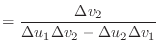
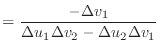
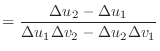
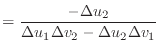
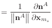
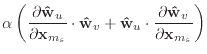
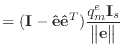
I derived equation (54) by the following logic. Define
![]() , and
, and
![]() . Then,
. Then,
![]() . Differentiating
. Differentiating ![]() , we obtain
, we obtain
and thus,

The derivation of (57) follows directly from differentation of this equation. In some ways, this definition feels a little circular due to the introduction of the artifical
I believe that there is a very small error in equation (14) of Baraff &
Witkin's paper: the ![]() term should be scaled by
term should be scaled by ![]() .
.
There is an error in their definition of
![]() , just above equation
(11). They define it as
, just above equation
(11). They define it as
However, the condition function
However, this yielded incorrect results, especially when calculating the damping forces for the bend condition, resulting in frequent instability. Later, I realised that correct application of the chain rule should yield a single
 |
(58) |
The final error in their paper is related to scale-invariance. Ideally, the
parameters used for the simulation should be independent of the tesselation of
the surface. For example, if you run the simulation with a
![]() mesh and a
mesh and a
![]() mesh and the same parameters, it should look
basically the same. However, using Baraff & Witkin's choice of
mesh and the same parameters, it should look
basically the same. However, using Baraff & Witkin's choice of ![]() ,
this does not occur. I looked at the math for the specific case where the
number of particles is doubled in
,
this does not occur. I looked at the math for the specific case where the
number of particles is doubled in ![]() and
and ![]() (e.g., from
(e.g., from
![]() to
to
![]() ). In this case, the gravity force on each original particle
decreases by a factor of four (since the mass of the surrounding triangles
decreases by four). However, the (strong) stretch and shear forces decrease by
a factor of eight. These forces are responsible for most of the resistance
against gravity, and consequently the cloth sags substantially as the particle
density is increased.
). In this case, the gravity force on each original particle
decreases by a factor of four (since the mass of the surrounding triangles
decreases by four). However, the (strong) stretch and shear forces decrease by
a factor of eight. These forces are responsible for most of the resistance
against gravity, and consequently the cloth sags substantially as the particle
density is increased.
However, by using
![]() , the stretch and shear forces also
decrease by a factor of four, as expected. The formula is not as intuitively
obvious as
, the stretch and shear forces also
decrease by a factor of four, as expected. The formula is not as intuitively
obvious as ![]() , and I have not done tests with irregularly triangulated
meshes, but it does work much better for regularly triangulated meshes.
, and I have not done tests with irregularly triangulated
meshes, but it does work much better for regularly triangulated meshes.
During my original development, I chased down one wrong alley while looking for the error in my (and Macri's) derivations. I was highly suspicious of one of Baraff & Witkin's approximations, where they assume that vectors' magnitudes are constant. This occurs in both the shear condition derivation and the bend condition derivation. I went through and rederived all of the formulas without this assumption, and obtained the formulas given in the appendix. After all of this work, there was still a problem, which proved to be the error in Macri's versions of equations (54) and (57).
After finding this error in Macri's work, I returned to the unit magnitude issue. I compared the results of my simulation using the formulas given in the body of the paper (using Baraff & Witkin's approximation) to the results using the formulas given in the appendix (without the approximation). In my test case, I found that the approximation gave more pleasing results! In total, stretch energy was halved, and shear and bend energy dropped by a small amount. The formulas for both stretch and bend energy are unchanged between the two cases, so this is a valid comparison of the energy in the cloth. The formula for shear energy is slightly changed by removing the unit magnitude approximation, however, so comparisons of energy aren't very meaningful.
To be honest, I was surprised that such a drastic change to the formulas had a relatively small effect on the final result. I suspect that there may be a lot of room for optimisation of Baraff & Witkin's system, achieving comparable results at less computational cost.
In the interests of presenting a direct implementation of Baraff & Witkin's paper, and on the basis of the better results, I have therefore presented the formulas with the constant magnitude approximation.
For parameters, I adopted values that gave good results. I looked at
Alias ![]() Wavefront's Maya cloth software, but I suspect that they scale
their parameters internally by an unknown amount. For damping forces, I
multiplied the associated regular force's constant by the damping constant
(e.g.
Wavefront's Maya cloth software, but I suspect that they scale
their parameters internally by an unknown amount. For damping forces, I
multiplied the associated regular force's constant by the damping constant
(e.g.
![]() was used to damp stretch forces).
was used to damp stretch forces).
|
To test out the simulator, I used a variety of cloth sizes and constraints. These can be seen at the Freecloth website http://davidpritchard.org/freecloth, in the screenshots section.
The simulator's performance is reasonable, with a
![]() cloth typically
requiring about thirty to forty minutes of computation per second of animation
on a 3 GHz Pentium IV system using a step size of
cloth typically
requiring about thirty to forty minutes of computation per second of animation
on a 3 GHz Pentium IV system using a step size of ![]() . Smaller cloth sizes
are much faster, and there is still a fair bit of room for optimisation,
especially in terms of adaptive timesteps.
. Smaller cloth sizes
are much faster, and there is still a fair bit of room for optimisation,
especially in terms of adaptive timesteps.
My implementation does exhibit some instability, but almost always works with a step size of 0.01 seconds; sometimes, a smaller stepsize is needed.
Baraff & Witkin's paper does indeed provide a solid framework for cloth simulation. It appears to allow relatively large timesteps, and with suitable optimisation should run quite quickly.
Hopefully, this paper should clear up some of the confusions of both Macri's paper, and the original paper. Implementing Baraff & Witkin's paper should be straightforward using the equations shown here.
This work was supported in part by a scholarship from the Natural Sciences and Engineering Research Council of Canada, and by the British Columbia Advanced Systems Institute.
Thanks to Sebastian Lipponer for pointing out a correction to the bend condition formulas.
The equations given in this appendix are replacements for certain equations given in the body of the paper. By using these, several of Baraff & Witkin's approximations are avoided. However, my tests show that the results are less pleasing.
 |
(A.1) | |
 |
(A.2) |
 |
 |
|
 |
(A.3) | |
 |
 |
|
 |
(A.4) |
If we remove the assumption that the
![]() and
and
![]() vectors are
unstretched, then equation (19) should be replaced with
vectors are
unstretched, then equation (19) should be replaced with
| (A.5) |
|
 |
(A.6) |
 |
 |
|
 |
(A.7) |
If we remove the assumption that the normal and edge vectors have constant length, we must replace equations (40) and (43) with those shown below.
 |
(A.8) | |
 |
(A.9) | |
 |
(A.10) |
|
||
 |
||
 |
||
 |
 |
||
 |
||
 |
||
 |
|
||
 |
||
 |
(A.11) |
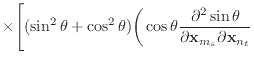
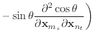
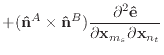
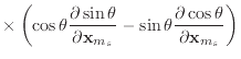
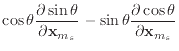
![$\displaystyle + 2 \sin\theta \cos\theta \left( \frac{\partial \cos \theta}{\par...
...bf x}_{m_s}} \frac{\partial \sin \theta}{\partial {\bf x}_{n_t}} \right) \Bigg]$](img189.png)